2  A new framework for personalized medicine: integrating

In the next few chapters we will show a new framework for personalized medicine. This is motivated by the fact that we know already some patients are more sensitive to endocrine therapy than others, but we don’t know what are possible treatments. Moreover, it is very difficult to compare, molecularly, patients among themselves.

The PREDICT tool (Wishart et al. 2010) provides a tool for practitioners to calculate survival risks among patients with similar clinical characteristics. This is very important as it shows how to combine data from previous patients to guide further treatments of new patients. However, no additional information is given, such as alternative pathways to target or what might be different from other patients.

Other tools that help in the clinics are the molecular signatures developed by companies (Wallden et al. 2015; Vijver et al. 2002; Paik et al. 2004). These signatures are intended to be used with ER+ BC patients and depending on the tool, on node negative, post-menopausal women. Based on the set of genes, a risk score is assigned or each patient. The score means if a patient would benefit from additional chemotherapy besides the usual endocrine therapy received for either 5 or 10 years. They also lack the additional information of what are possible pathways involved and alternative treatments beside chemotherapy.

There are a few challenges to overcome pathway analysis for patients individually and how to compare patients molecularly. There is no tool that allows to integrate patients in a continuous way. Usually integration is a one step procedure and cannot be updated. The usual tools are (Risso et al. 2014; Zhang, Parmigiani, and Johnson 2020; Fei et al. 2018) and they do not provide batch effect removal for new samples. The only way is to re-run the procedure together with the new sample. The problem of doing this is usually you don’t have enough samples to estimate batch effects across groups and therefore correct it.

This chapter show how to perform PCA projection using samples from different datasets and how new samples can be introduced without retraining of the PCA. We first introduce the notion of a new normalization that depends on housekeeping genes. After using this new normalization, we proceed with PCA on a subset of two cohorts using the 1000 most variable genes. We then validate the integration with new samples from a completely different cohort.

* The library is already synchronized with the lockfile.

    ../../results/plots/pca_merging ../../results/rds_files/pca_merging 
                              FALSE                               FALSE 
   ../../results/tables/pca_merging 
                              FALSE 

2.1 Transcriptomics and qPCR normalization

In this first step we introduce a new normalization. The rational is that we need a normalization procedure that is applied in a single sample only, similar to logCPM, but that can be applied to microarray too. In this case, given a set of samples, we start by ranking the genes in each sample. We then normalize the ranking to be between 0 and 1, i.e., we divide by the total number of genes available in that sample. Then, given a list of 50 stable genes across cancer (Bhuva, Cursons, and Davis 2020), we calculate the average ranking of these genes in the sample and then for each gene in the sample we divide by this average.

2.1.1 Selecting stable genes

The first step is to check what number of these 50 genes are available on TCGA and METABRIC, as these datasets will be used for training the PCA projection. The total number of available genes is 44. Table 2.1 shows the name of the genes available in TCGA and METABRIC.

Now we select the 1000 most variable genes across METABRIC and TCGA. Reducing the number of genes used when calculating the PCA helps in the future. Several publicly available datasets don’t have many genes available, therefore reducing the number of genes increases the chances of using this approach in other datasets.

Moreover, the use of a large number of genes is used because if some of them are not available. We show in later sections that if some number of stable genes are missing, it will not affect the normalization.

Figure 2.1: (Table 2.1) Available stable genes in both TCGA and METABRIC cohorts.

2.1.2 Calculating the normalization

We will create subset of the summarised experiment objects to save these information. Moreover, since a summarized experiment object is being used, we can save the new normalization in the assays and the average ranking scores of the housekeeping genes in the column data colData. This way it is very easy to retrieve the information for the patients.

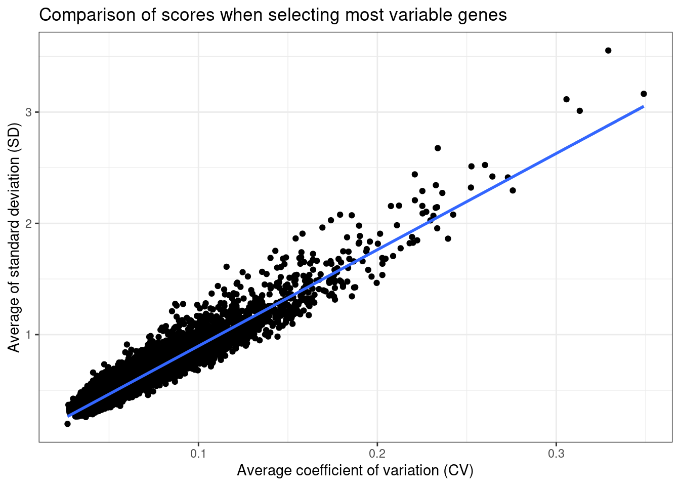
Figure 2.2: Comparison of coefficient of variation and standard deviation scores.

They are highly correlated values, so we stick to the coefficient of variation as it makes more sense in this kind of analysis.

Table 2.3 shows the top 1000 genes along with their standard deviation. The stable genes are also added to the list.

Figure 2.3: (Table 2.3) Standard deviation of each gene in each condition and pooled standard deviation.

Overall we can see that housekeeping genes have very low standard deviation across cohorts, which is good.

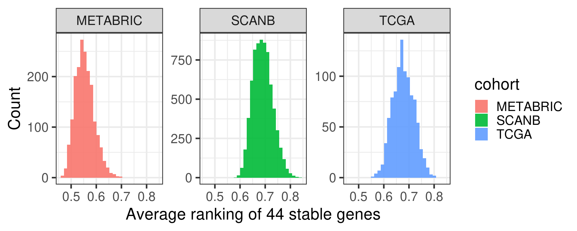
Figure 2.4 shows a histogram with the distribution of the average ranking of the housekeeping genes for each sample in each cohort.

Figure 2.4: Distribution of the average ranking of the housekeeping genes defined previously for each cohort separately.

The average ranking are somewhat similar. For the two experiments where there are RNA-seq samples, the distribution is the same. For METABRIC, a microarray experiment, the distribution is shifted a bit below.

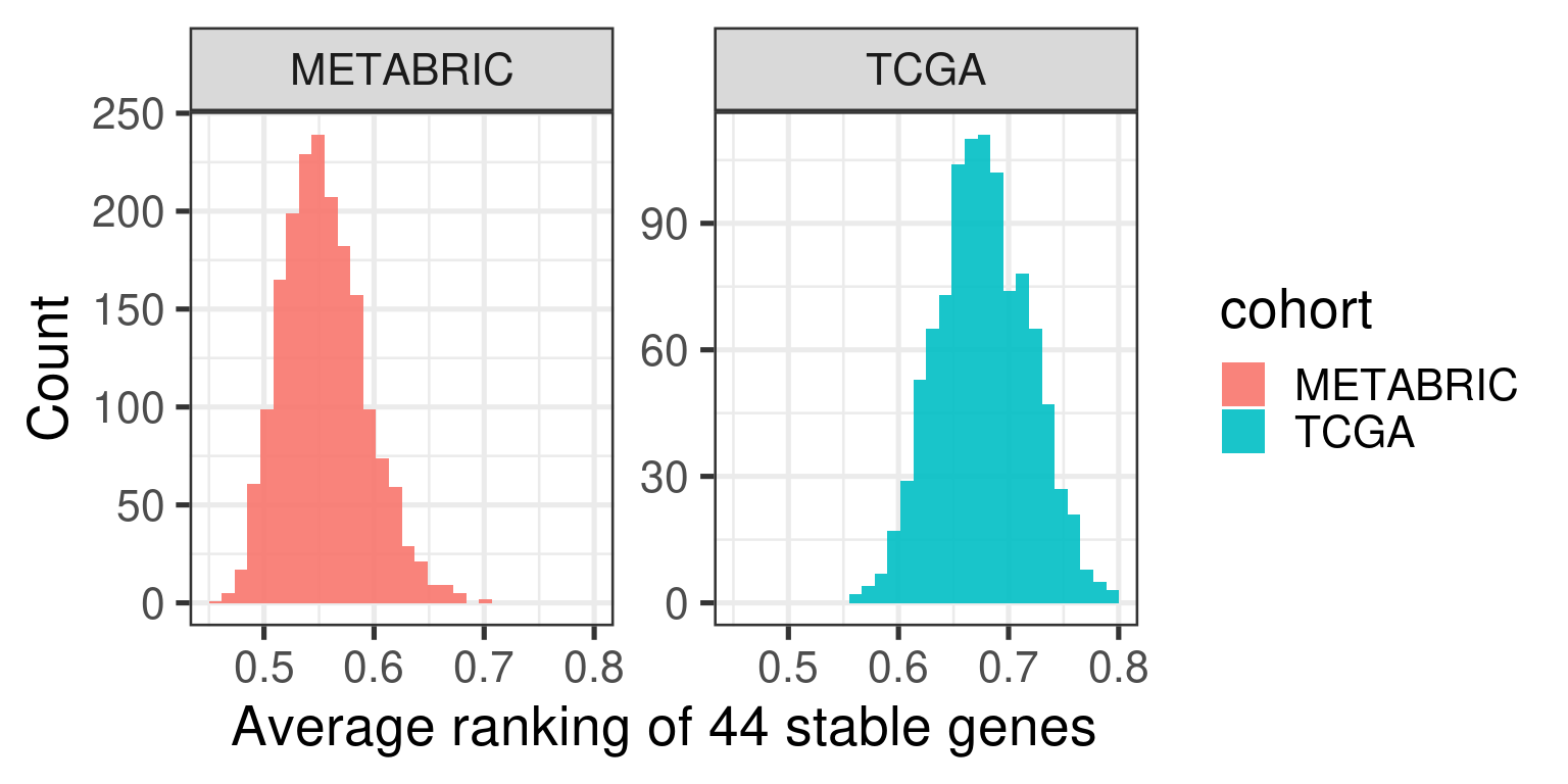
Figure 2.5: Distribution of the average ranking of the housekeeping genes defined previously for each cohort separately.

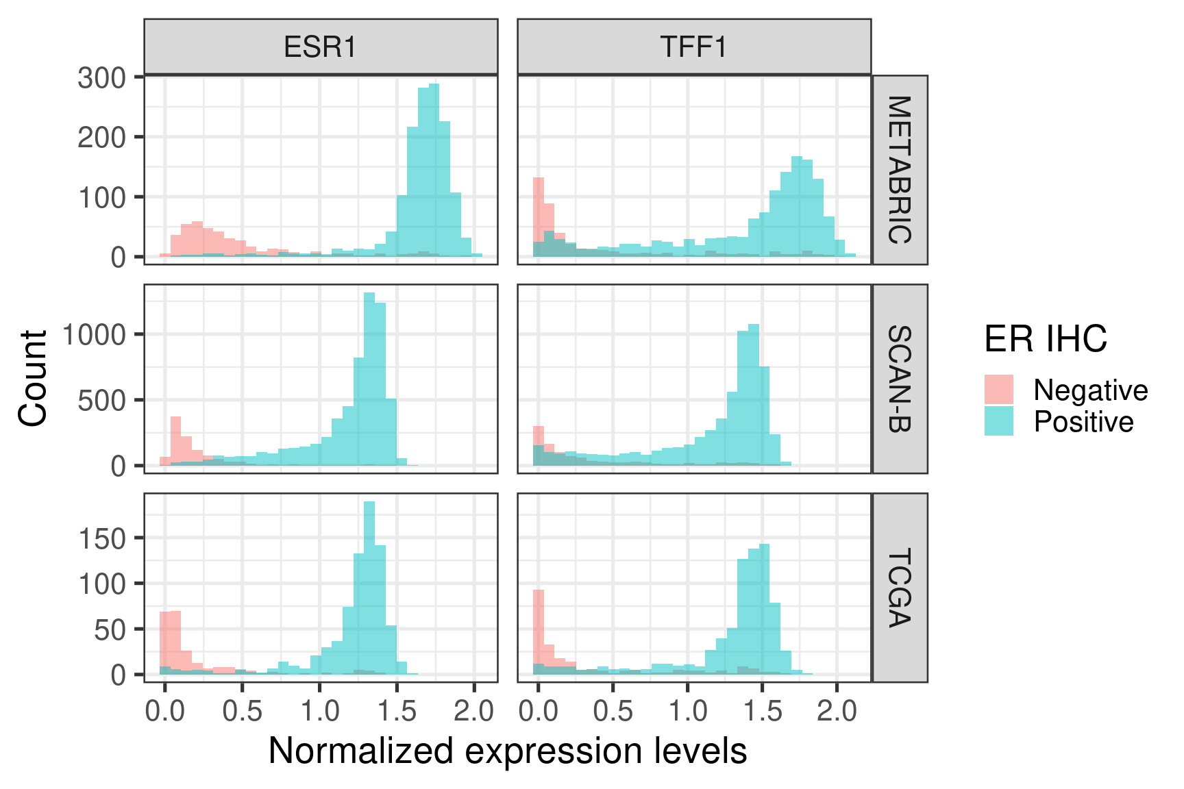
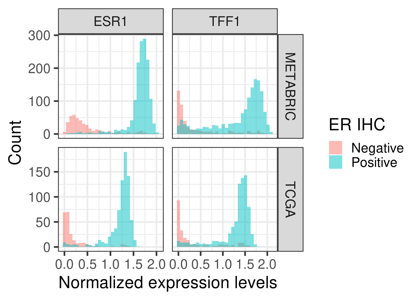
Figure 2.6 shows histograms of gene expression from some important genes in breast cancer.

Figure 2.6: Distribution of the gene expression levels of ESR1 and TFF1 in each one of the cohorts

ESR1 and TFF1 expressions are divided across ER status, as expected.

Figure 2.7: Distribution of the gene expression levels of ESR1 and TFF1 in each one of the cohorts

The numbers of samples available for each cohort are shown in the table below.

   cohort      Negative      Positive         Total
 METABRIC  4.3%   (429) 14.3% (1,439) 18.5% (1,868)
   SCAN-B 10.5% (1,059) 61.0% (6,157) 71.5% (7,216)
     TCGA  2.3%   (231)  7.7%   (774) 10.0% (1,005)

2.1.3 Checking robustness with respect of number of stable genes available

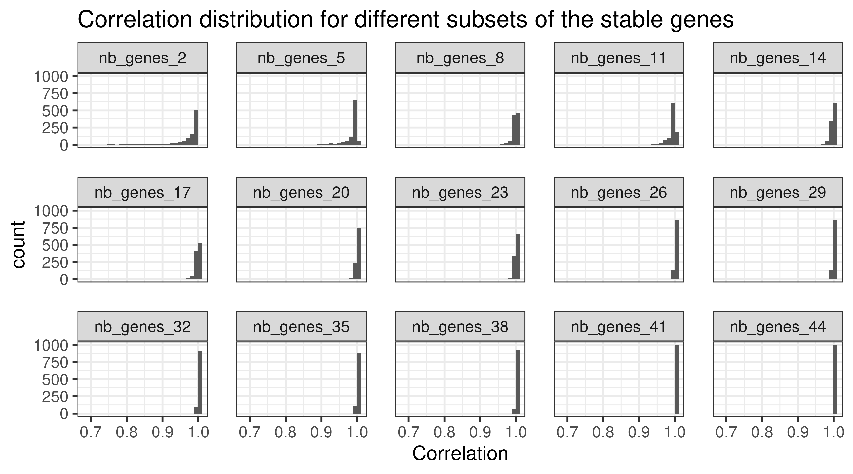
When calculating the normalized data, a total of 44 stable genes were used. Sometimes not all of these genes are available, therefore we will calculate the normalization using random subsets of 44 stable genes with different random sizes. The sets will have a minimum of 20 genes and maximum of 44. The sampling of the set size is obtained by using a uniform distribution. We focus just on TCGA for simplicity. The correlation used in this case was the Pearson correlation.

Figure 2.8: Correlation distribution for different subsets of housekeeping genes (HKGs). Each different subset has a different number of HKGs.

Figure 2.8 shows the different distributions given the subsets of housekeeping genes. All the correlation coefficients are close to 1. This means that if a subset of housekeeping genes are missing it is fine, as the others will compensate.

Figure 2.9

2.2 Integrating TCGA and METABRIC using PCA

The next step is creating the framework where we can integrate any patient sample and compare each other, at least spatially. The approach is similar to some sort of unsupervised learning, where no labels or groups are specified, which is something common in algorithms for batch removal. By using PCA in some subset of TCGA and METABRIC, we should learn the idiosyncrasies of the RNA-seq and microarray technologies as well as batch effects general to datasets. Since these two cohorts are big ones, we assume that if there are common batch effects, they are represented on them.

The practical steps are: first subselect 1000 samples in total from METABRIC and TCGA. Train PCA using these 1000 samples. Validate the results by projecting the other samples. In the next section we show how robust the approach is when selecting the samples. In the next chapters we validate the projection in unseen cohorts.

Integrating as laid out here only uses molecular data, therefore patients might be close to each other but they might have very different clinical features. This should always be kept in mind.

The table below shows the molecular characteristics of the patients selected for the PCA training.

cohort	basal	her2	lumb	luma	normal	claudin-low	Total
metabric	7.3% (73)	7.4% (74)	16.3% (163)	22.4% (224)	4.6% (46)	6.8% (68)	64.8% (648)
tcga	7.0% (70)	2.8% (28)	6.1% (61)	17.7% (177)	1.6% (16)	0.0% (0)	35.2% (352)
Total	14.3% (143)	10.2% (102)	22.4% (224)	40.1% (401)	6.2% (62)	6.8% (68)	100.0% (1,000)

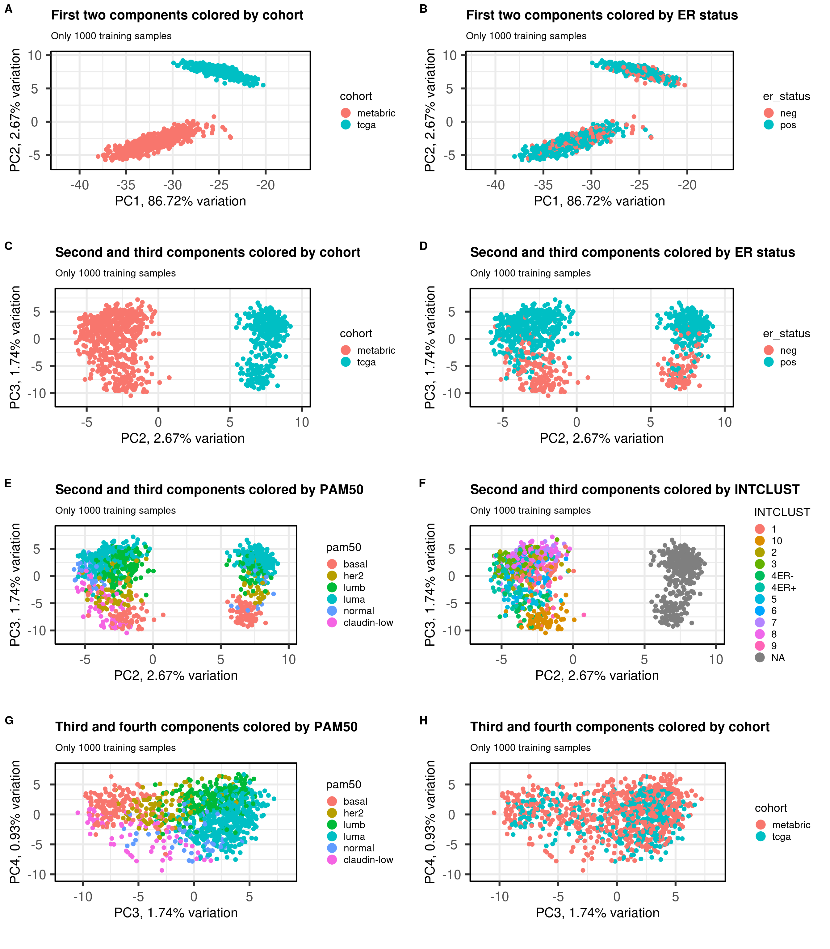
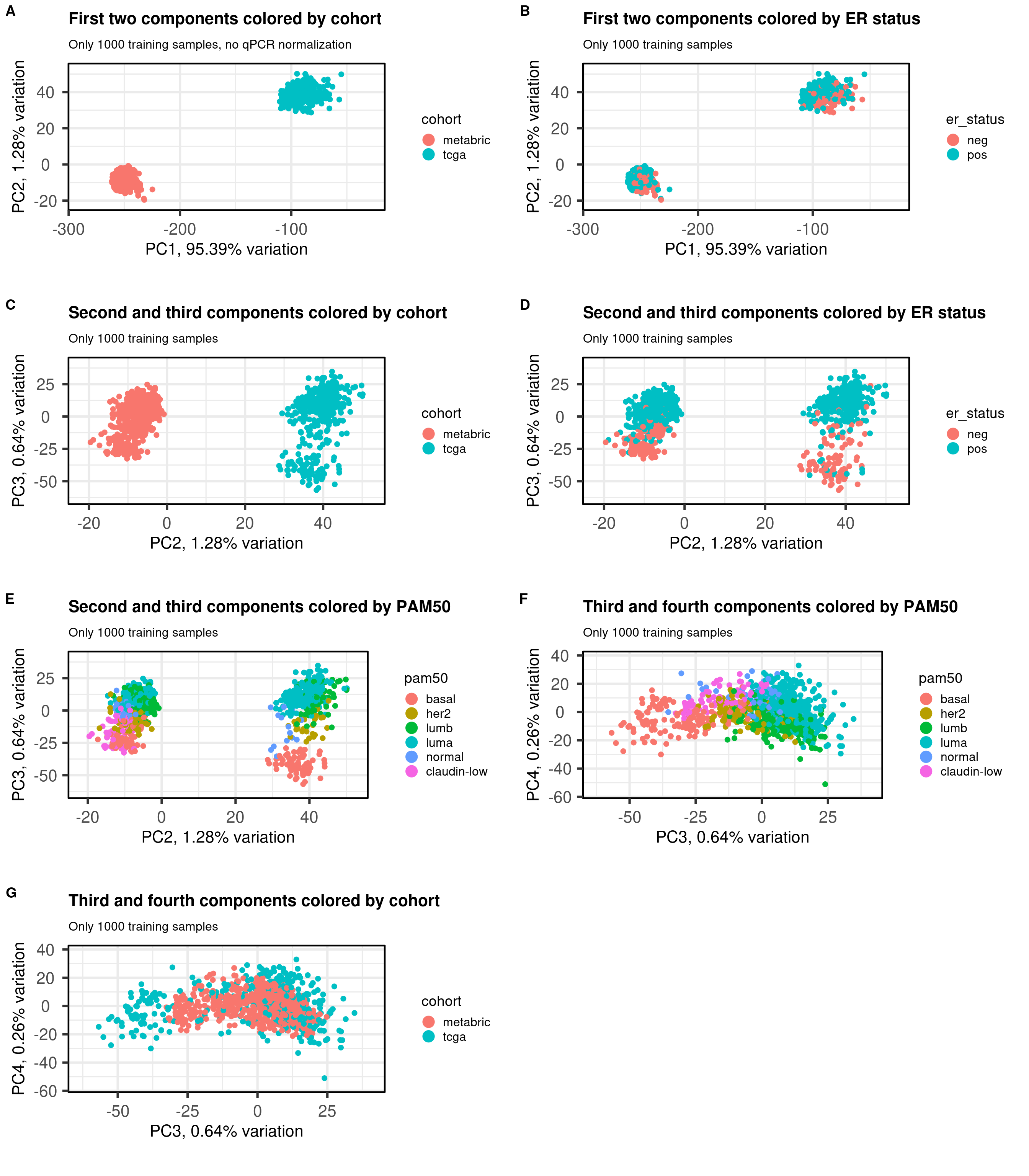
Figure 2.10 shows the embedding of the two datasets together of the 1000 samples used for training. We select several PCs of interest to show how the embedding works.

Figure 2.10: PCA projections colored by different factors and organized by different components. (A) Plot of the first two components colored by cohort. (B) Plot of the first two components colored by ER status. (C) Plot of the second and third components colored by cohort. (D) Plot of the second and third components colored by ER status. (E) Plot of the second and third components colored by PAM50. (F) Plot of the second and third components colored by INTCLUST, only METABRIC has an assigned value for this variable, NAs are TCGA samples.

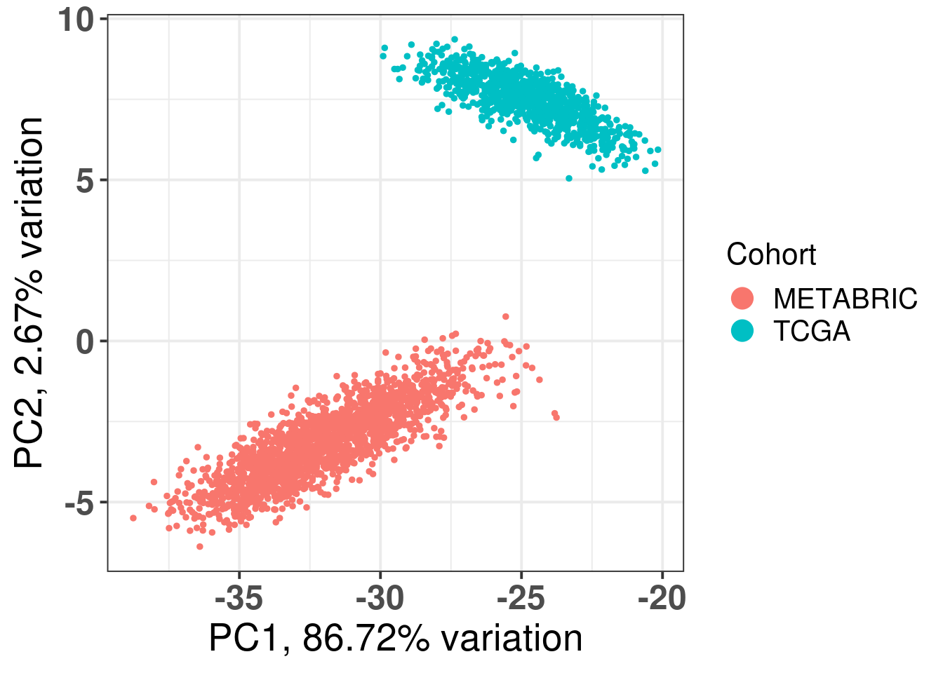
The first three components correspond to the batch effect. The third component explains the ER status and the two cohorts are well inter mingled. When plotting the third and fourth components and coloring by the molecular subtype, we see a clear distinction, recapitulating the biology.

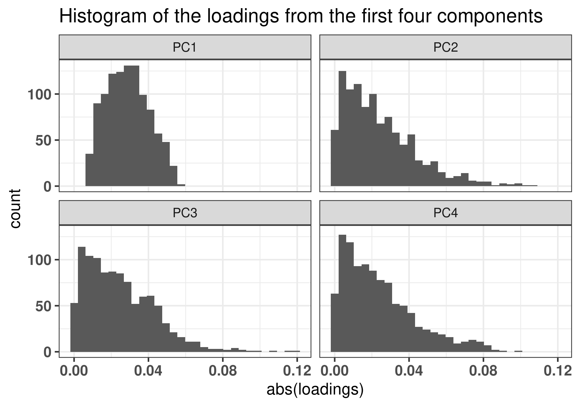
The plot below shows how the loadings of the first component are really concentrated around zero, so there are not actually specific genes that are accounting for the batch effects we see in the first component. We show latter that the genes that are the most important are the ones with high loading, so the tail of the distributions. In this sense there are really no genes in the tail of the loadings for PC1.

Figure 2.11: Different loadings for the first 4 components.

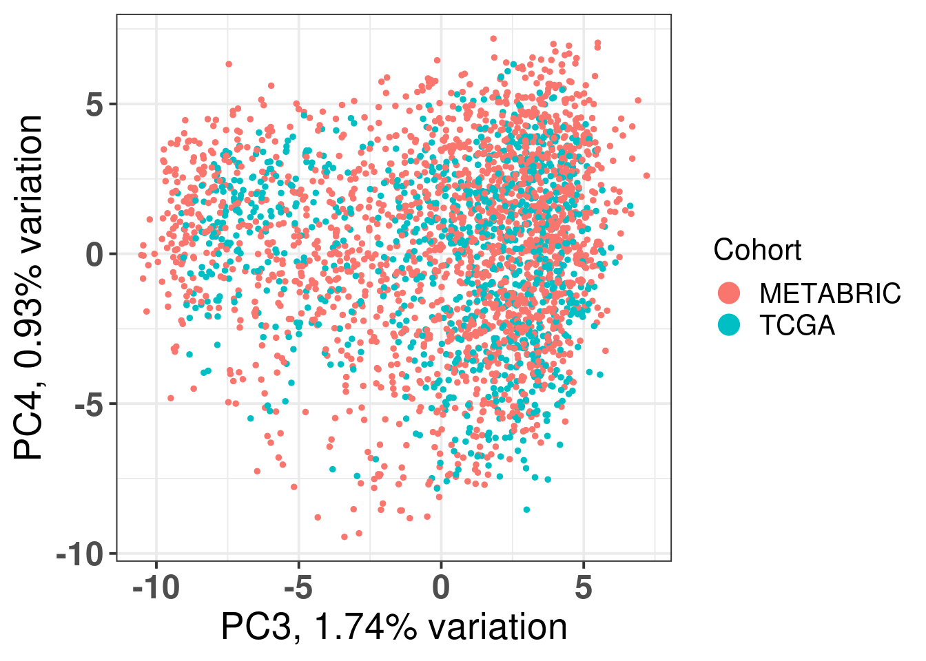
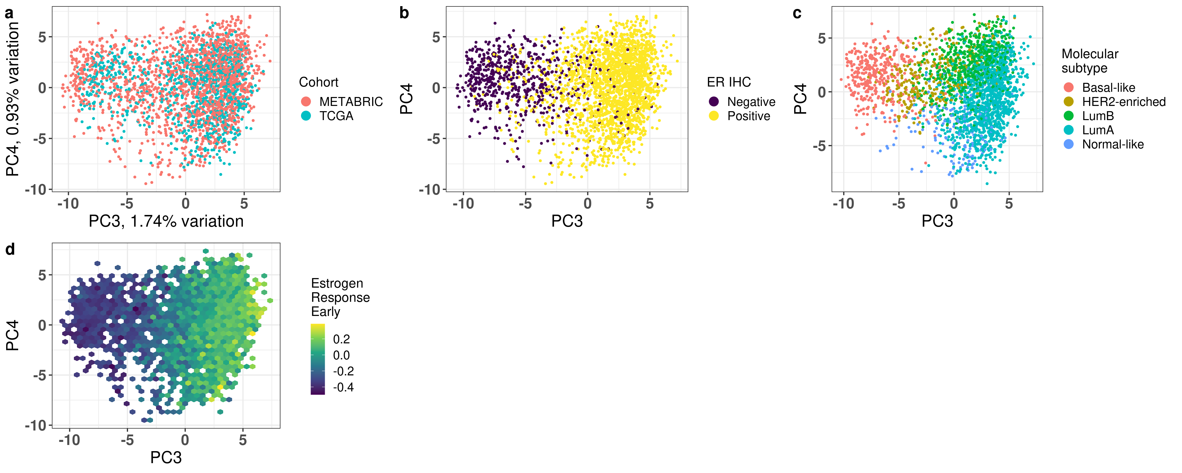
Figure 2.12 shows all the samples from TCGA and cohort projected into the molecular landscape.

Figure 2.12: Original PC3 and PC4 of all samples, including test and train samples, of TCGA and METABRIC.

And the first two PCs.

Figure 2.13: Original PC1 and PC2 of all samples, including test and train samples, of TCGA and METABRIC.

And Figure 2.14.

Figure 2.14: Original PC3 and PC4 of all samples, including test and train samples, of TCGA and METABRIC.

In order to check if the integration made sense, it is possible to color by ER status, NPI for METABRIC samples and tumor/node stage for TCGA. To check ER signaling scores, the pathways Estrogen response early/late and \(SET_{ER/PR}\) are used to color the projection.

Figure 2.15 shows the coloring by age.

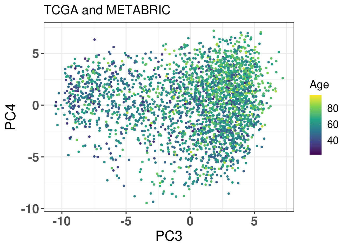
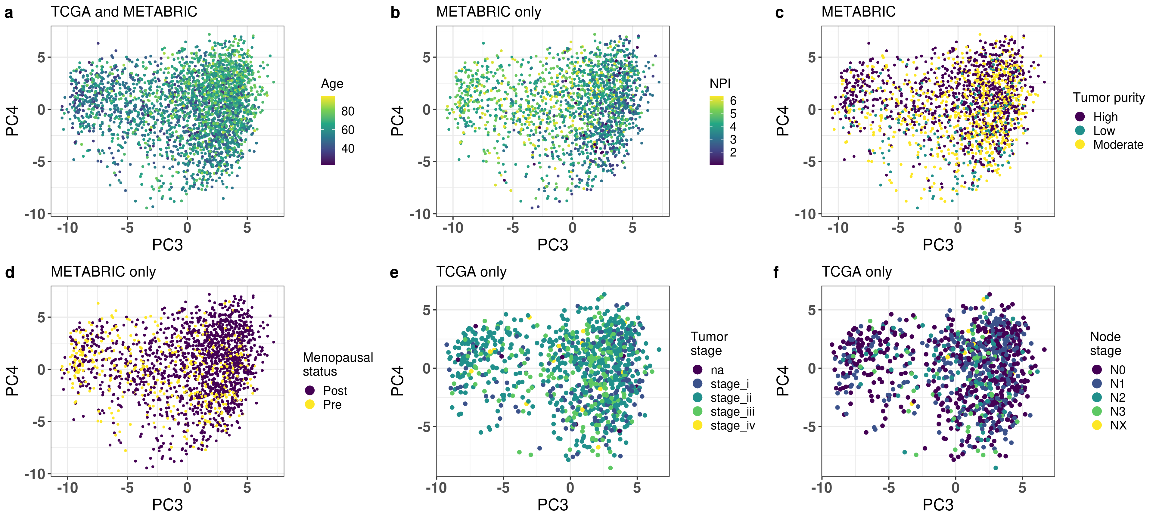
Figure 2.15: PC3 and PC4 of samples from TCGA and METABRIC colored by age.

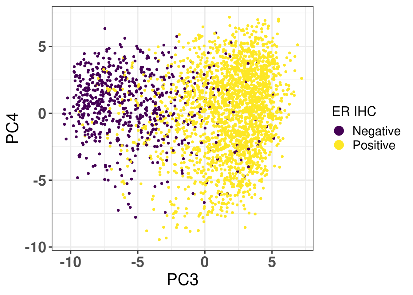
Age seems to be well mixed. Figure 2.16 shows the PCA colored by ER status.

Figure 2.16: PC3 and PC4 of samples from TCGA and METABRIC colored by ER status.

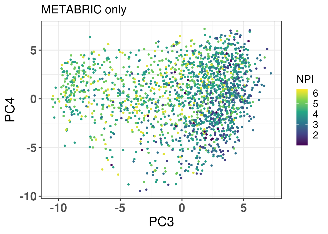
It has a very good separation among the different patients. Figure 2.17 is the PCA embedding colored by NPI. Only METABRIC samples have this information.

Figure 2.17: PC3 and PC4 of samples from METABRIC only colored by NPI.

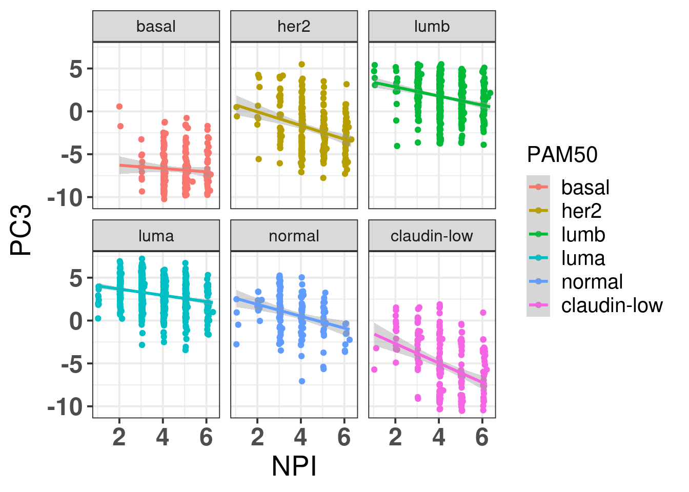
It looks good, ER+ BC patients have lower NPI, which makes sense. Figure 2.18 shows then how there is barely any correlation between the different subtypes and the NPI when stratified by the molecular subtype.

Figure 2.18: PC3 and NPI correlation colored and stratified by the intrinsic molecular subtype.

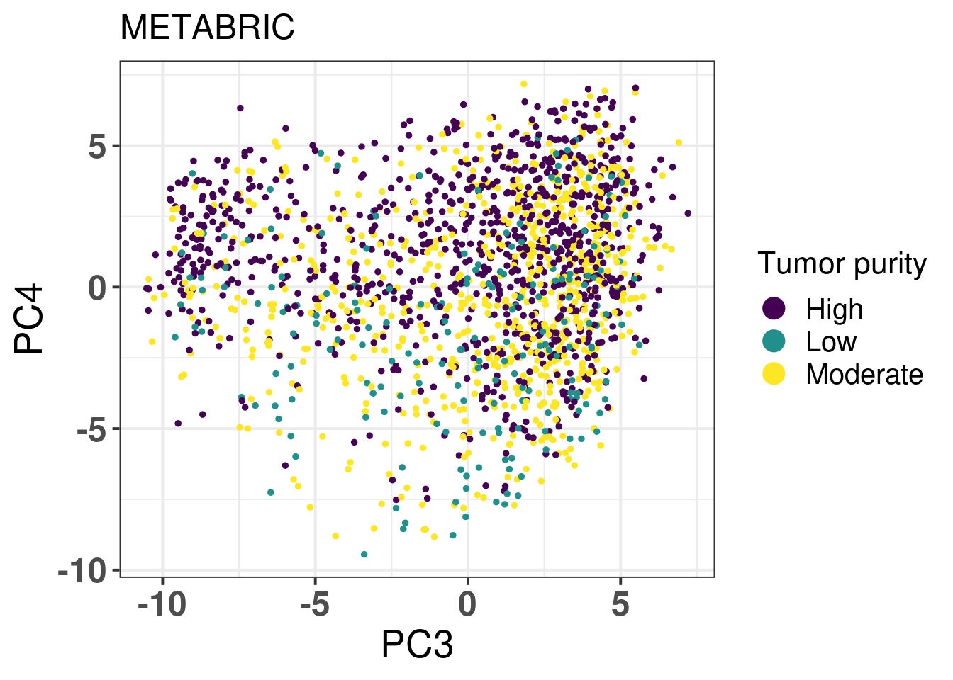
Figure 2.19 shows the biplot colored by tumor purity.

Figure 2.19: PC3 and PC4 of samples from METABRIC only colored by tumor purity.

The tumor purity is not a factor that is affecting the embedding as samples with low cellularity (< 40% of tumor cells) and high cellularity (> 70% of tumor cells) intermingle.

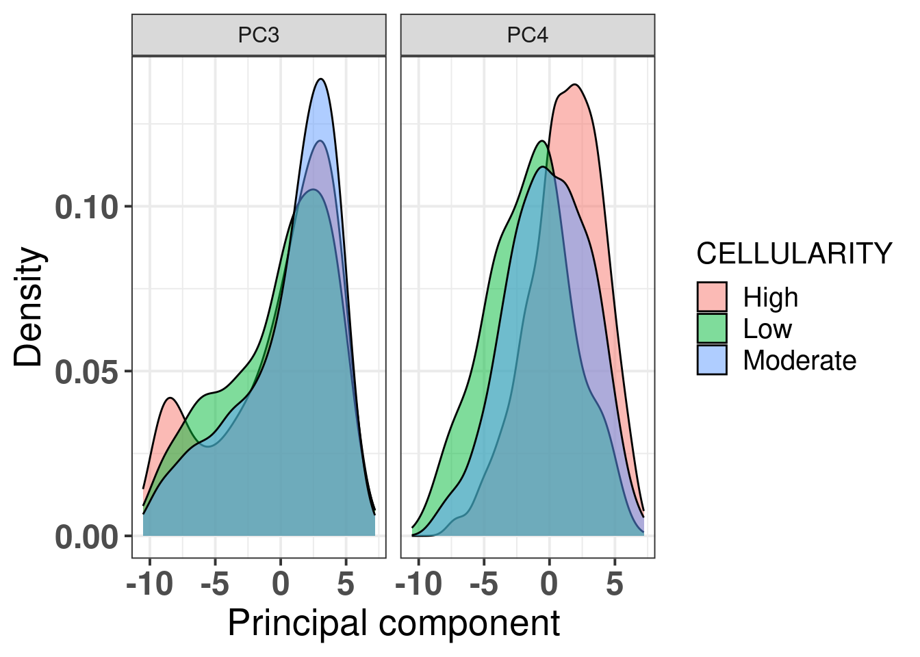
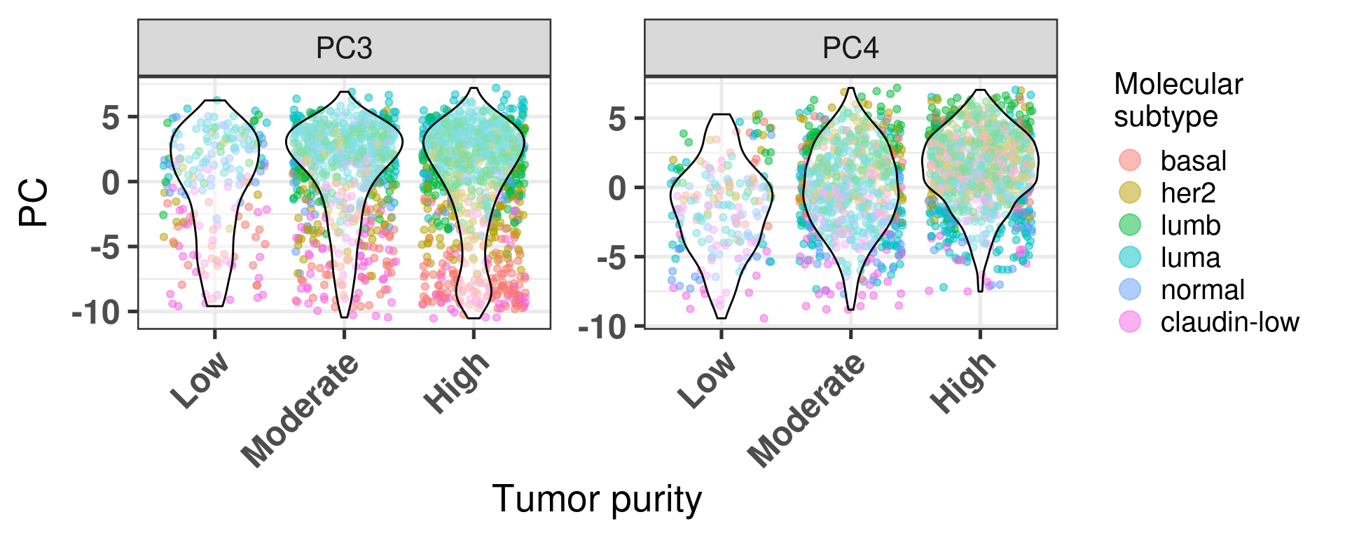
Another way to visualize is the distribution of the principal components over the tumor purity (Figure 2.20).

Figure 2.20: PC3 and PC4 stratified by tumor purity

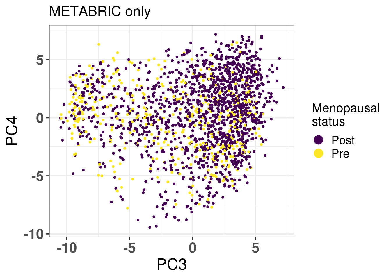
METABRIC has also inferred menopausal status for the patients, we use this information to check if there is any enrichment based on the patient menopausal status (Figure 2.21)

Figure 2.21: PC3 and PC4 of samples from METABRIC only colored by menopausal status.

We don’t see any difference between the two status. We proceed now with the analysis using clinical factors from TCGA.

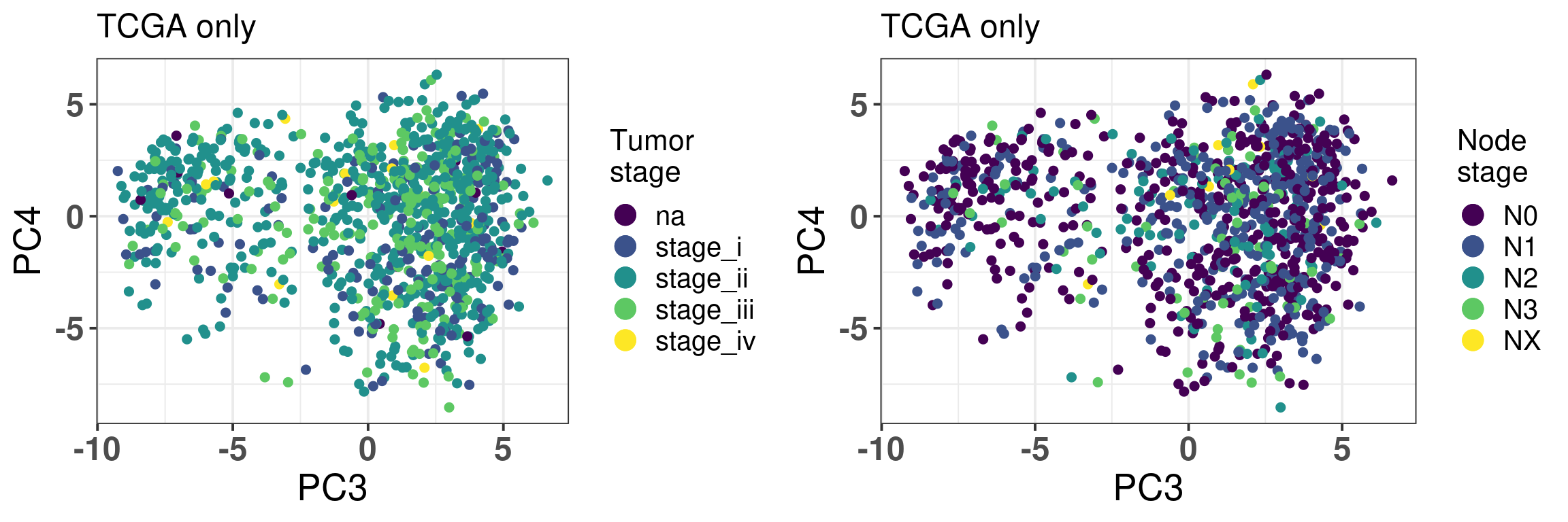
Figure 2.22: PC3 and PC4 of samples from TCGA only colored by tumor stage and node stage.

For both tumor and node stage the samples seem to have mixed well, indicating the projection is not a function of the stages, as shown in Figure 2.22.

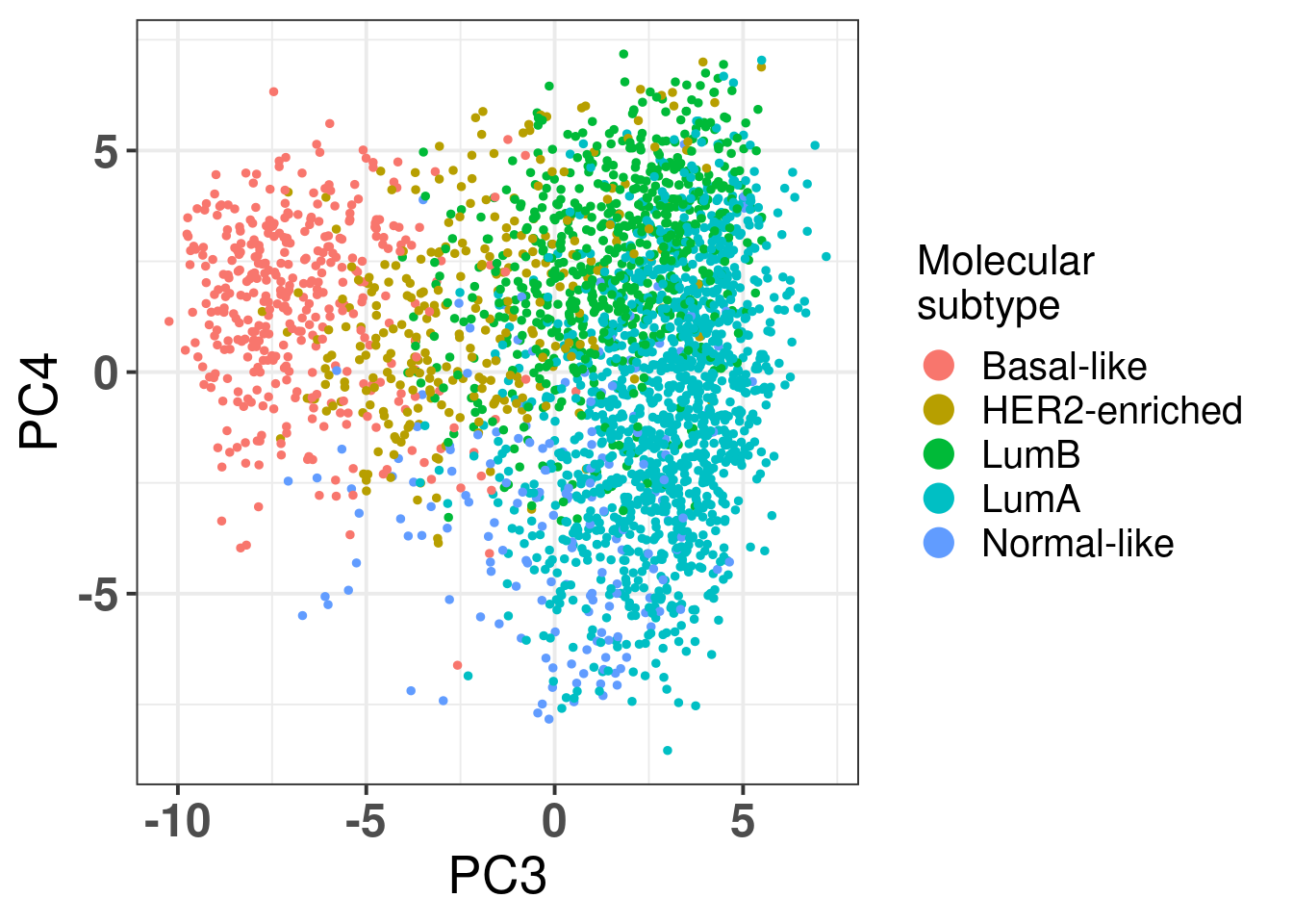
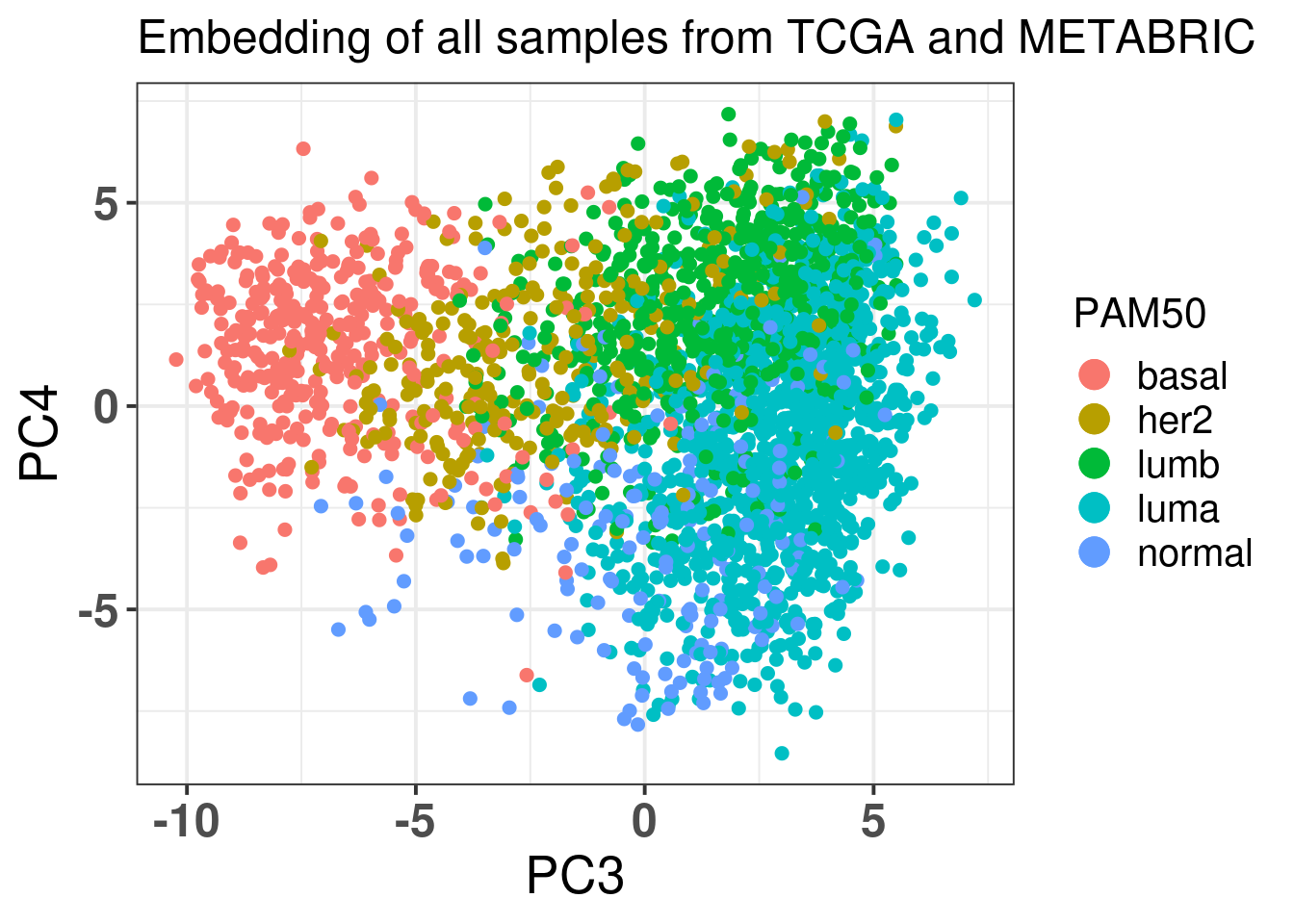
And finally Figure 2.23 below shows the color by PAM50 molecular subtype.

Figure 2.23: Corrected PC3 and PC4 of samples from TCGA and METABRIC colored by PAM50 molecular subtype.

The molecular subtypes are projected as expected, going from left to right there are the basal-like BC patients, going to HER2 and then they are split between luminal A and B. The normal like patients are in the top and closer to the luminal A, reflecting the biology.

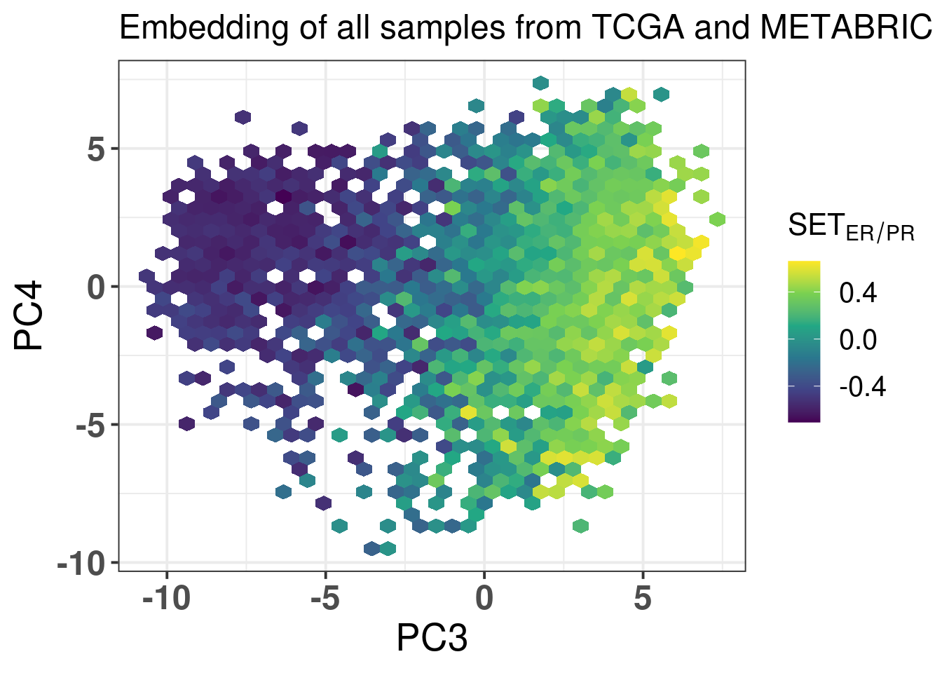
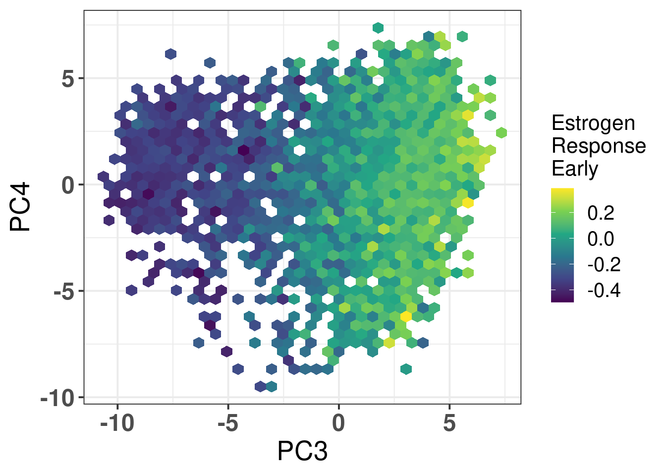
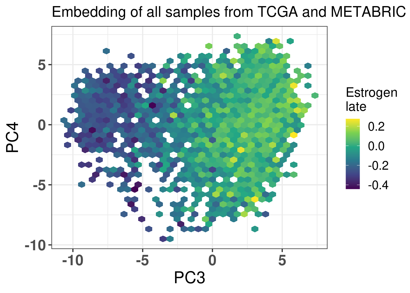
The next figures show the ER signaling measures coloring the projections.

Figure 2.24: biplot of PC3 and PC4 of samples from TCGA and METABRIC colored by the SET ER/PR score.

Figure 2.25: biplot of PC3 and PC4 of samples from TCGA and METABRIC colored by the hallmark estrogen response early.

Figure 2.26: biplot of PC3 and PC4 of samples from TCGA and METABRIC colored by the hallmark estrogen response late

In all cases the mixing is relatively good. For \(SET_{ER/PR}\) you have a gradient going from the right to the left, showing again that patients on the far top right probably are those patients with better prognosis.

And we now display the plots together to include in the first figure of the paper.

Figure 2.27

And now we also plot by age (TCGA and METABRIC), NPI, tumor purity and menopausal state (METABRIC only) and Node stage (TCGA only) all combined for the supplementary figure of the paper.

Figure 2.28

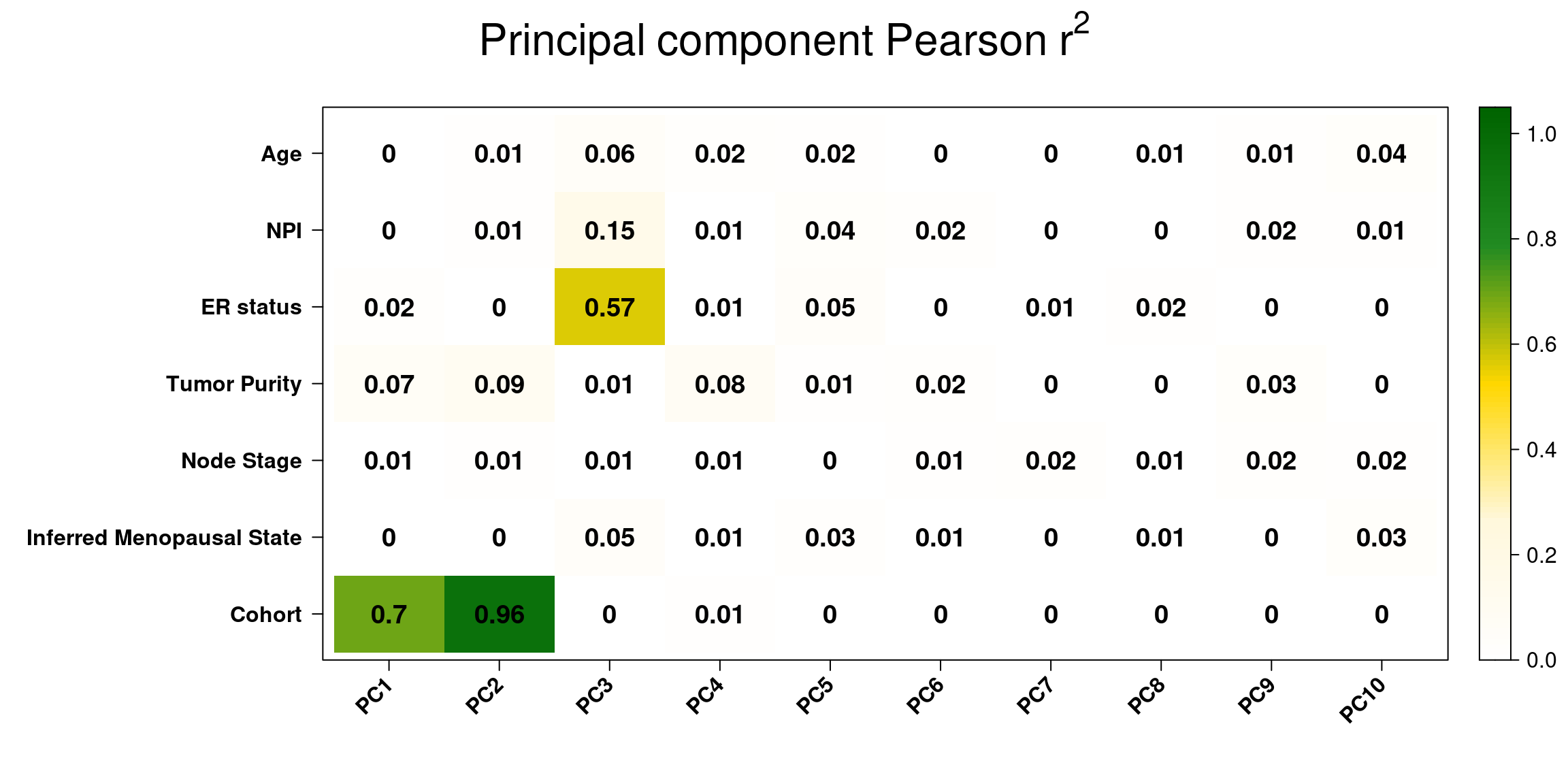
And lastly we use the correlation plot available from PCAtools to check the PC correlation with all the clinical factors, we check the first 10 components as these are the ones with more variation.

Figure 2.29: Pearson r-squared between clinical factors and principal components.

We see that the two biggest correlations is with cohort and PC1/PC2 as expected. There is a bit of correlation of NPI and PC3, since basal-like tumors have usually higher NPI scores, they are more aggressive. Also, as expected ER status has a pretty high correlation with PC3 since the basal like are on the left of the principal component and the luminal A/B are on the right region.

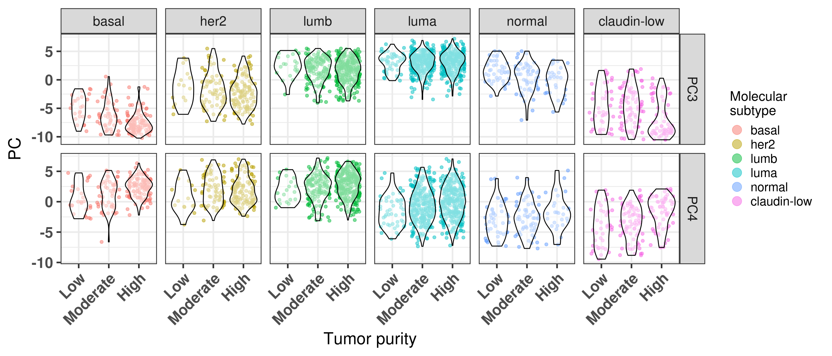
Moreover, basal-like tumors are more pure compared to the luminal A. For the luminal A subtype the amount of tumors that are high or moderate in terms of purity are balanced (around 45%). In all subtypes, the amount of samples with low tumor purity are overall low, excluding the normal-like and claudin-low.

CELLULARITY	basal	her2	lumb	luma	normal	claudin-low
High	60.5% (118)	59.0% (121)	63.1% (281)	47.6% (315)	21.9% (28)	33.7% (61)
Low	12.8% (25)	7.3% (15)	4.5% (20)	7.4% (49)	34.4% (44)	22.7% (41)
Moderate	26.7% (52)	33.7% (69)	32.4% (144)	45.0% (298)	43.8% (56)	43.6% (79)
Total	100.0% (195)	100.0% (205)	100.0% (445)	100.0% (662)	100.0% (128)	100.0% (181)

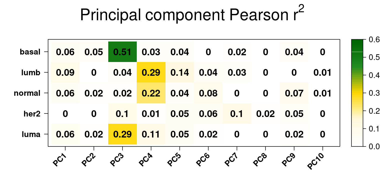
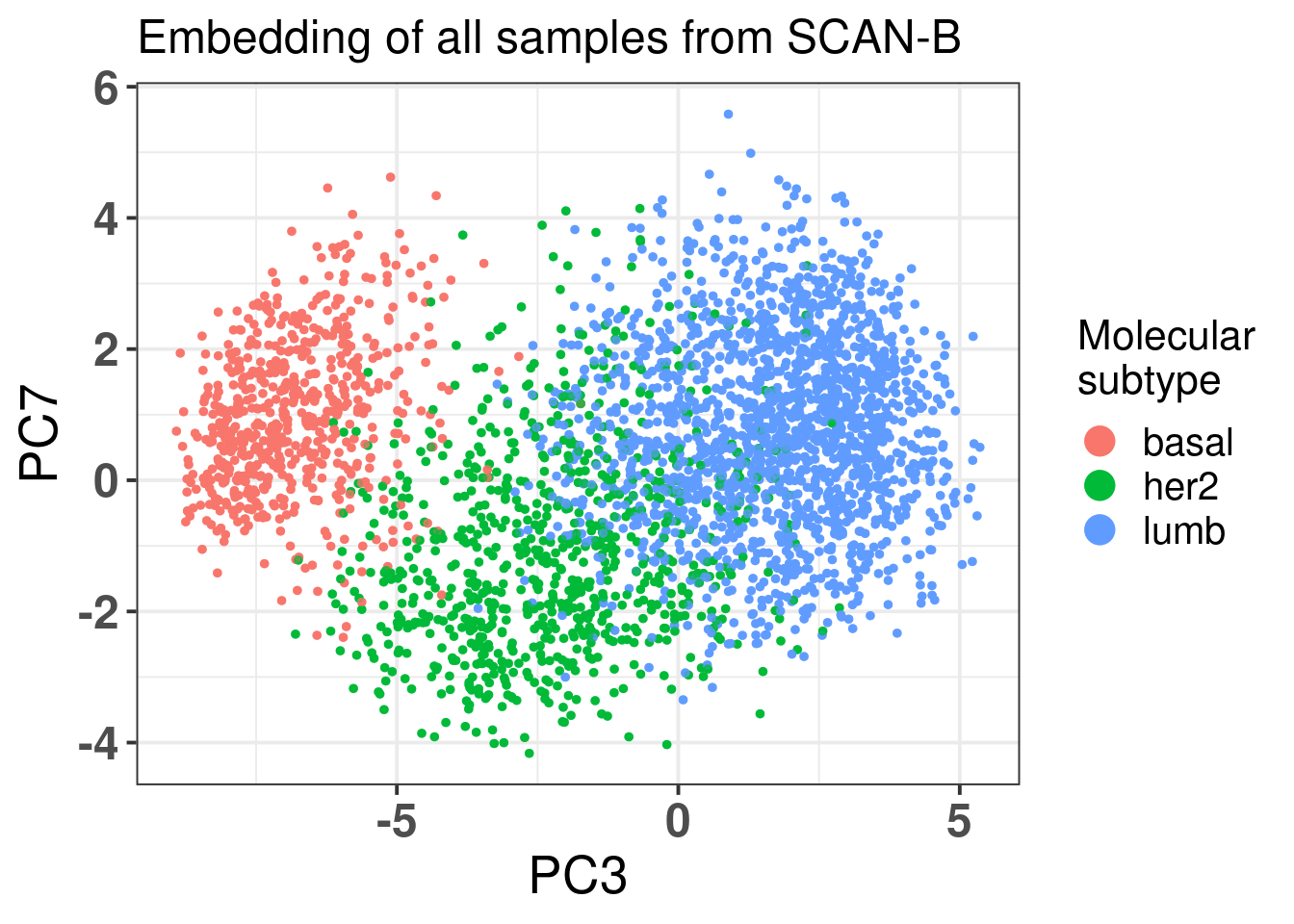
Next we just show the \(r^2\) pearson residuals for the SCAN-B, an external cohort.

Figure 2.30

We see that the majority of the residuals are explained in PC3 and PC4, as expected. The HER2 seems to have a similar correlation in PC3 and PC7. Below we plot only basal-like, luminal B and HER2 enriched tumor samples to compare.

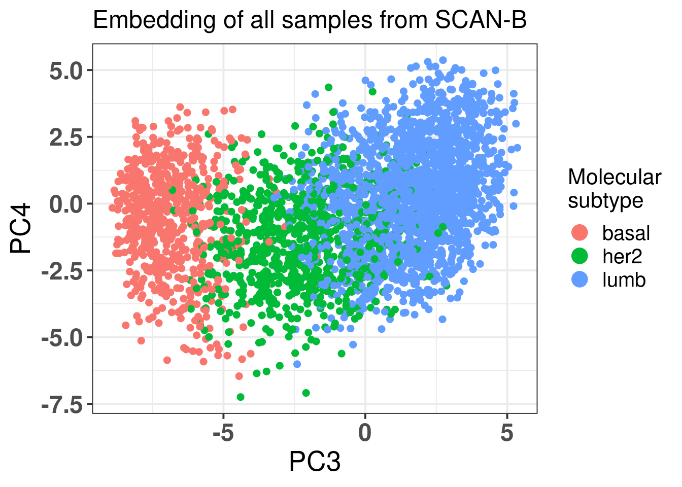
In fact the difference is mainly on PC3 and not so much on PC7. It is only a subset of those samples that have lower PC7. And when we compare PC3 vs PC4.

PC7 is not adding much in general to the separation.

2.3 The integration is robust with respect of selection of samples

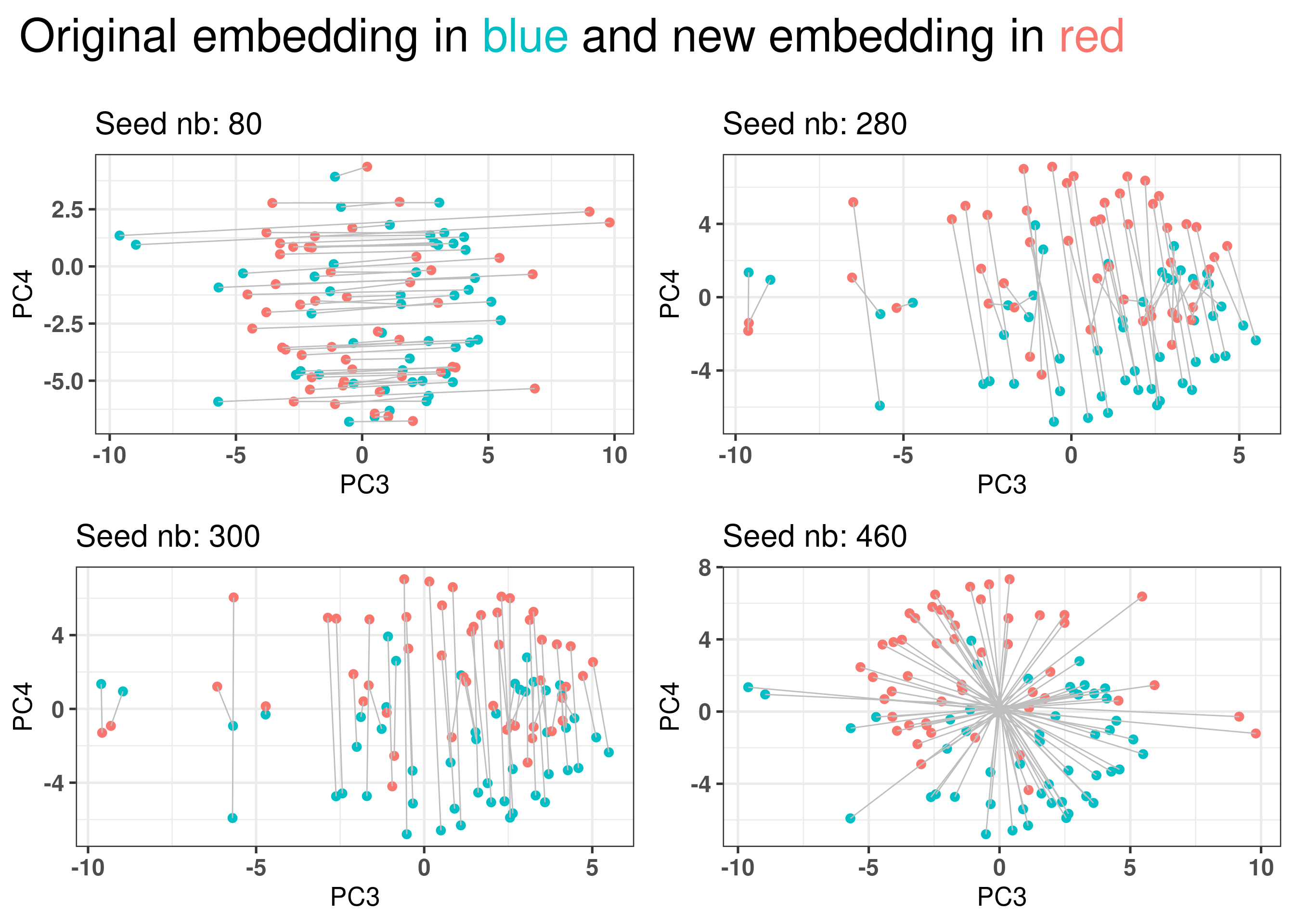
The embedding could be due to the patients selected and samples that are close to each other in one embedding would be far away from them in another embedding. Ten random sets of 1000 patients are sampled and the embedding is calculate. A total of 10 PCA embeddings are obtained.

Figure 2.31: Selecting a random set of 1000 patients an rerunning the pipeline to obtain other embeddings. Red color corresponds to the embedding using the new fitted PCA. Blue corresponds to the embedding of the original PCA. Each dot corresponds to a patient.

Figure 2.31 shows that the embedding is invariant for rotation, translation and reflection for 4 random sets of samples coming from either METABRIC or TCGA.

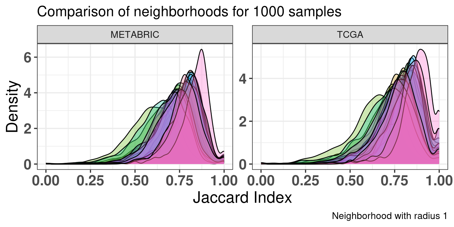
Figure 2.32 shows the jaccard index distributions for each cohort separately when comparing the sample neighborhoods of the new embeddings with the original embedding. The jaccard index is counting the number of samples in the intersection of the neighborhoods in the original and the new embedding divided by the total number of unique samples in both neighborhoods. A high value means a good agreement with the neighborhoods.

A thousand samples were randomly selected from each cohort individually and the jaccard index for each new embedding was calculated.

Figure 2.32: Jaccard index distribution for 1000 samples in each cohort individually. Each color corresponds to a different seed and embedding, with a total of 18 seeds.

And below we show the standard deviation of the average of the distributions.

# A tibble: 1 × 2
  mean_of_jaccard_mean sd_of_jaccard_mean
                 <dbl>              <dbl>
1                0.747             0.0605

This indicates a high agreement.

2.4 Normalization is necessary to reduce batch effects in other components

Since PCA is removing batch effects from the datasets, one could argue it could also remove platform dependent normalization values and therefore one would need to look only at lower principal components. In this section we show that doing the normalization is necessary to get a good integration in the datasets.

The idea is similar as before, but instead of performing the qPCR-like normalization on the datasets, one would use the logFPKM values for TCGA and median intensity for microarray. The problem with this kind of approach also includes the fact that only other samples that went through this processing could be used in the pipeline.

Figure 2.33: PCA projections colored by different factors and organized by different components. (A) Plot of the first two components colored by cohort. (B) Plot of the first two components colored by ER status. (C) Plot of the second and third components colored by cohort. (D) Plot of the second and third components colored by ER status. (E) Plot of the second and third components colored by PAM50.

Figure 2.33 shows the contrast with the other method including the normalization. Without the normalization, the samples from METABRIC tend to concentrate close to the center, they are not so well mixed.

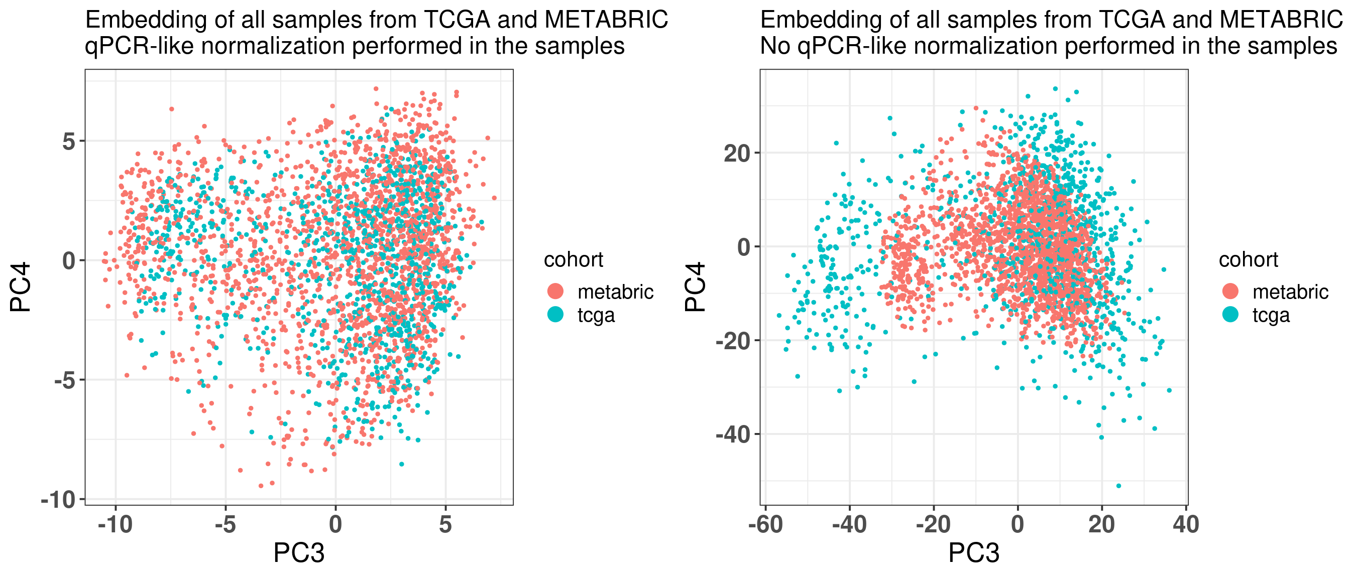
Figure 2.34: PC3 and PC4 from all METABRIC and TCGA samples. (A) Embedding using the qPCR-like normalization. (B) Embedding using the original normalization from each dataset.

Figure 2.34 shows side by side the differences when using the qPCR-like normalization and when not using. The left plot is using the qPCR normalization and shows how well the mixing gets, putting samples in the same scale. If the scaling in a sample level is not performed, samples do not mix well.

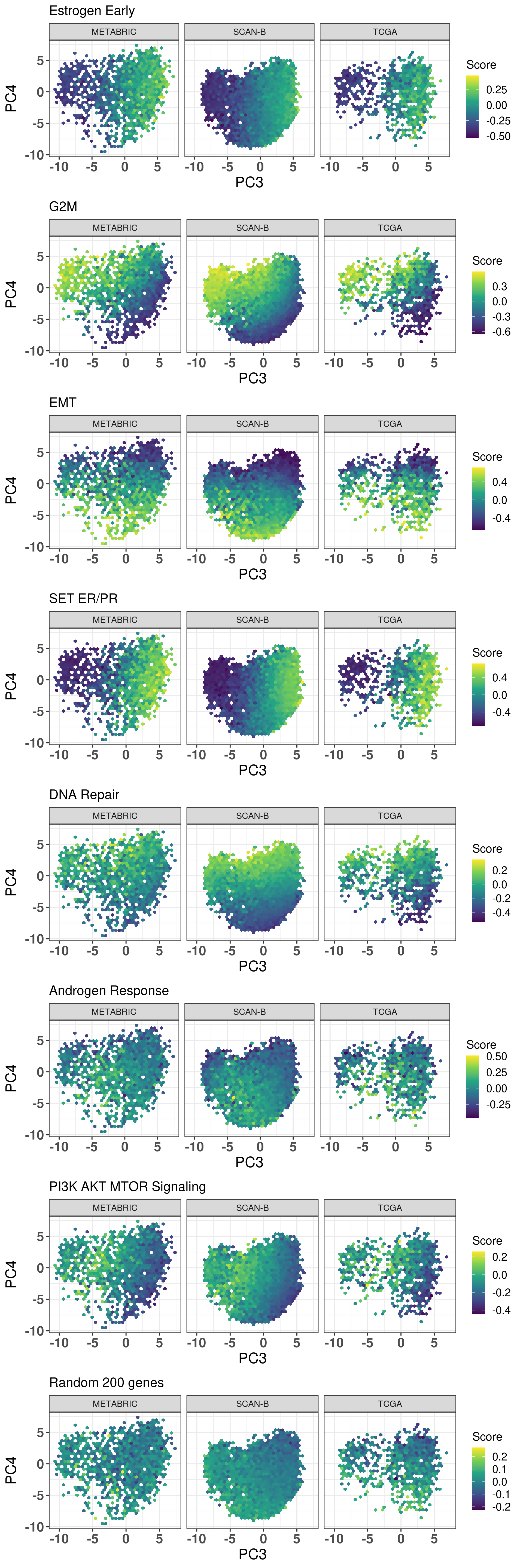
2.5 Molecular landscape is characterized by several pathways

Among the 1000 genes that are used when calculating the molecular landscape, several might be involved in biological process. Figure 2.35 shows that several pathways are associated with the position in the molecular landscape. Something that is particularly remarkable here is the association of the epithelial mesenchymal transition and DNA repair pathways with PC4.

Figure 2.35: Hex biplots colored by different pathways. Each hex is colored based on the average score in the hex.

We see that these pathways are somehow relevant to the embedding, but are they also prognostic of overall survival in the two cohorts? In the next chunks we evaluate this hypothesis. Mostly the focus is on ER+ BC patients that received some kind of hormonal therapy. As seen before, for the TCGA dataset we select ER+ BC patients that have the molecular subtype luminal A and B instead.

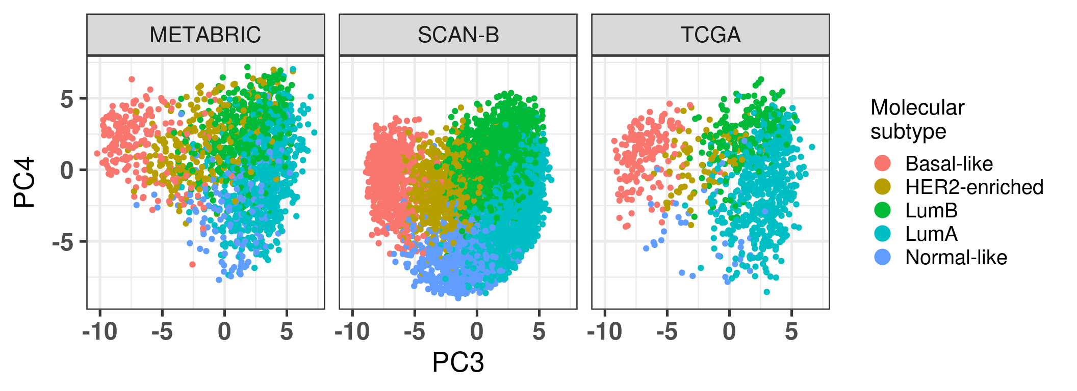
Just before moving on we plot the embedding colored by molecular subtype stratified by cohort so it can go together with a figure in the paper and it is easier to compare the pathways.

Figure 2.36

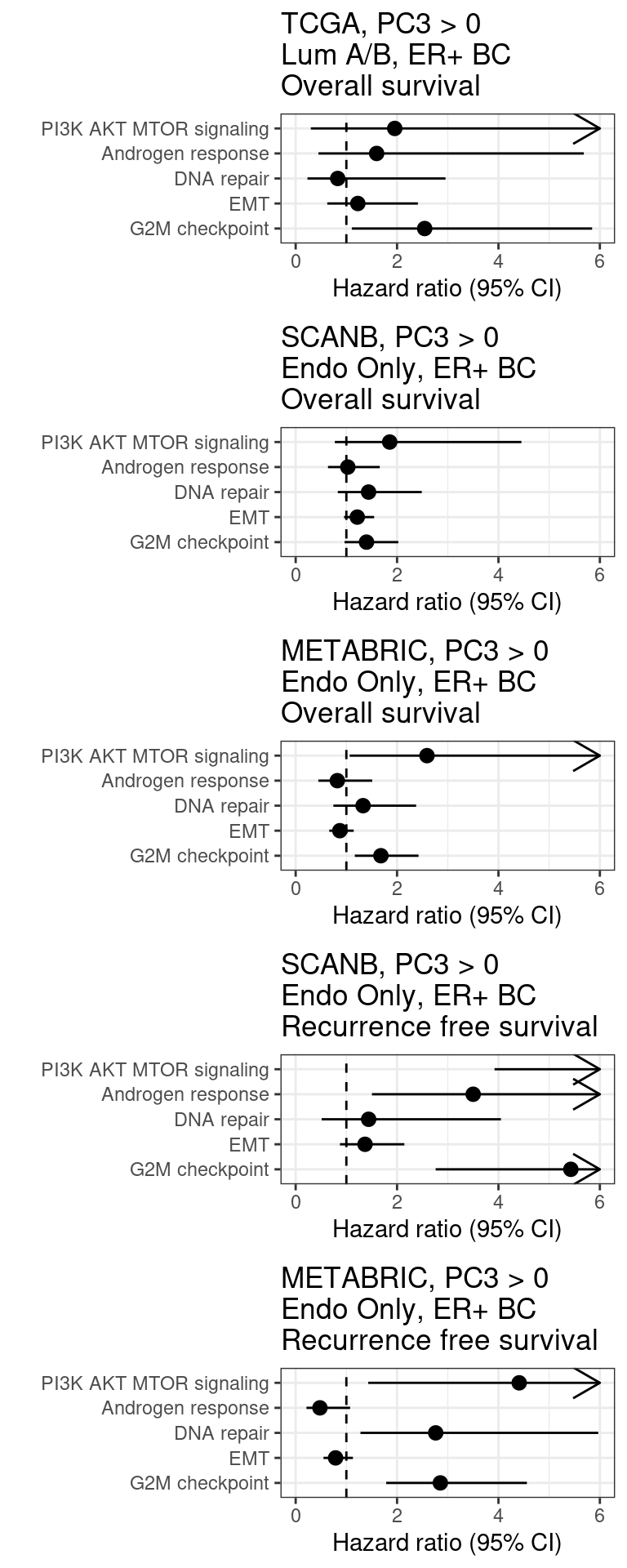
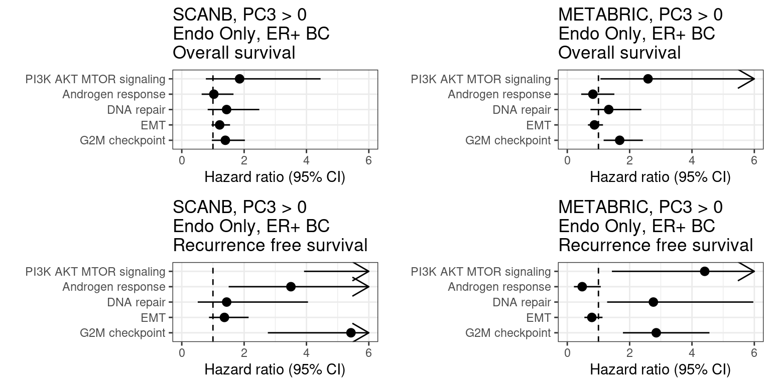
Figure 2.37: Overall survival analysis from all the three big cohorts and their scores. The formulas used were the same as for the estrogen signaling analysis.

We see that G2M checkpoint has hazard ratio higher than 1. The other scores are a bit more variable and can change the sign (type S error).

Figure 2.38: Overall survival analysis from all the three big cohorts and their scores. The formulas used were the same as for the estrogen signaling analysis.

Below is the table with the scores.

2.6 Tumor Purity

One possible problem that might arise in the analysis is the tumor purity. We showed already the molecular embedder colored by tumor purity but here we look more carefully at the relationship between PC3 and PC4 with tumor purity as made available by METABRIC.

We actually compare the PC3 and PC4 with tumor purity stratified by molecular subtype, as it is expected that the normal-like subtype is correlated with lower tumor purity.

And when we look at all subtypes together.

Overall there is an absence of evidence that tumor purity is affecting PC3 and PC4 in a systematic way.

Bhuva, Dharmesh D, Joseph Cursons, and Melissa J Davis. 2020. “Stable Gene Expression for Normalisation and Single-Sample Scoring.” Nucleic Acids Research 48 (19): e113–13. https://doi.org/10.1093/nar/gkaa802.

Fei, Teng, Tengjiao Zhang, Weiyang Shi, and Tianwei Yu. 2018. “Mitigating the Adverse Impact of Batch Effects in Sample Pattern Detection.” Edited by Inanc Birol. Bioinformatics 34 (15): 2634–41. https://doi.org/10.1093/bioinformatics/bty117.

Paik, Soonmyung, Steven Shak, Gong Tang, Chungyeul Kim, Joffre Baker, Maureen Cronin, Frederick L. Baehner, et al. 2004. “A Multigene Assay to Predict Recurrence of Tamoxifen-Treated, Node-Negative Breast Cancer.” New England Journal of Medicine 351 (27): 2817–26. https://doi.org/10.1056/nejmoa041588.

Risso, Davide, John Ngai, Terence P Speed, and Sandrine Dudoit. 2014. “Normalization of RNA-Seq Data Using Factor Analysis of Control Genes or Samples.” Nature Biotechnology 32 (9): 896–902. https://doi.org/10.1038/nbt.2931.

Vijver, Marc J. van de, Yudong D. He, Laura J. van t Veer, Hongyue Dai, Augustinus A. M. Hart, Dorien W. Voskuil, George J. Schreiber, et al. 2002. “A Gene-Expression Signature as a Predictor of Survival in Breast Cancer.” New England Journal of Medicine 347 (25): 1999–2009. https://doi.org/10.1056/nejmoa021967.

Wallden, Brett, James Storhoff, Torsten Nielsen, Naeem Dowidar, Carl Schaper, Sean Ferree, Shuzhen Liu, et al. 2015. “Development and Verification of the PAM50-Based Prosigna Breast Cancer Gene Signature Assay.” BMC Medical Genomics 8 (1). https://doi.org/10.1186/s12920-015-0129-6.

Wishart, Gordon C, Elizabeth M Azzato, David C Greenberg, Jem Rashbass, Olive Kearins, Gill Lawrence, Carlos Caldas, and Paul DP Pharoah. 2010. “PREDICT: A New UK Prognostic Model That Predicts Survival Following Surgery for Invasive Breast Cancer.” Breast Cancer Research 12 (1). https://doi.org/10.1186/bcr2464.

Zhang, Yuqing, Giovanni Parmigiani, and W Evan Johnson. 2020. “ComBat-Seq: Batch Effect Adjustment for RNA-Seq Count Data.” NAR Genomics and Bioinformatics 2 (3). https://doi.org/10.1093/nargab/lqaa078.