1  Estrogen receptor status is continuous, not dichotomous

Currently in the clinics estrogen receptor (ER) status is treated as dichotomous condition. Either a breast cancer (BC) is ER positive (ER+) or ER negative (ER-). The threshold for ER+ cells usually is 1% or 10% of the cells positive in a IHC staining. The idea is that ER+ BC patients will receive endocrine therapy, usually tamoxifen or some aromatase inhibitor, for treatment. The problem is not all patients respond the same to these drugs and they also have different proportions of ER+ cells.

In this document we show how leveraging molecular information distinguishes ER+ BC patients and how one should look more carefully on ER status. In order to do this, estrogen related signatures: estrogen response early and late from MSigDB(Subramanian et al. 2005) and \(SET_{ER/PR}\)(Sinn et al. 2019), are used to calculate scores for each BC patient. These scores then are used to calculate associations with survival analysis. When performing cox regression, we try to adjust for sensible covariates in order to reduce bias. Even though we are adjusting, it is very difficult to know if a covariate is missing in the regression. Thus, care should be always taken when interpreting these results.

This chapter is structure in the following way. First section corresponds to loading the datasets and then filtering them. Estrogen signatures scores are calculated using GSVA (Hänzelmann, Castelo, and Guinney 2013). Given the scores, cox regression can be performed adjusting for clinical variables. After this the Hazard ratios can be computed and interpreted along with their confidence intervals.

1.1 Loading and filtering the datasets

The preprocessing of the datasets is described in the website below: > https://chronchi.github.io/transcriptomics

To check the code used here either click in the code button on the top right part of the page or check the github page (github.com/chronchi/molecular_landscape).

The TCGA, METABRIC and SCANB cohorts are used in this section here. They are the biggest cohort of Breast cancer patients in the world. Each datasets has an overall equal distribution of ER+ and ER- patients and similar age distribution.

* The library is already synchronized with the lockfile.

    ../../results/plots/surv_analysis_estrogen 
                                         FALSE 
../../results/rds_files/surv_analysis_estrogen 
                                         FALSE 
   ../../results/tables/surv_analysis_estrogen 
                                         FALSE 

1.2 UMAP embedding of the datasets

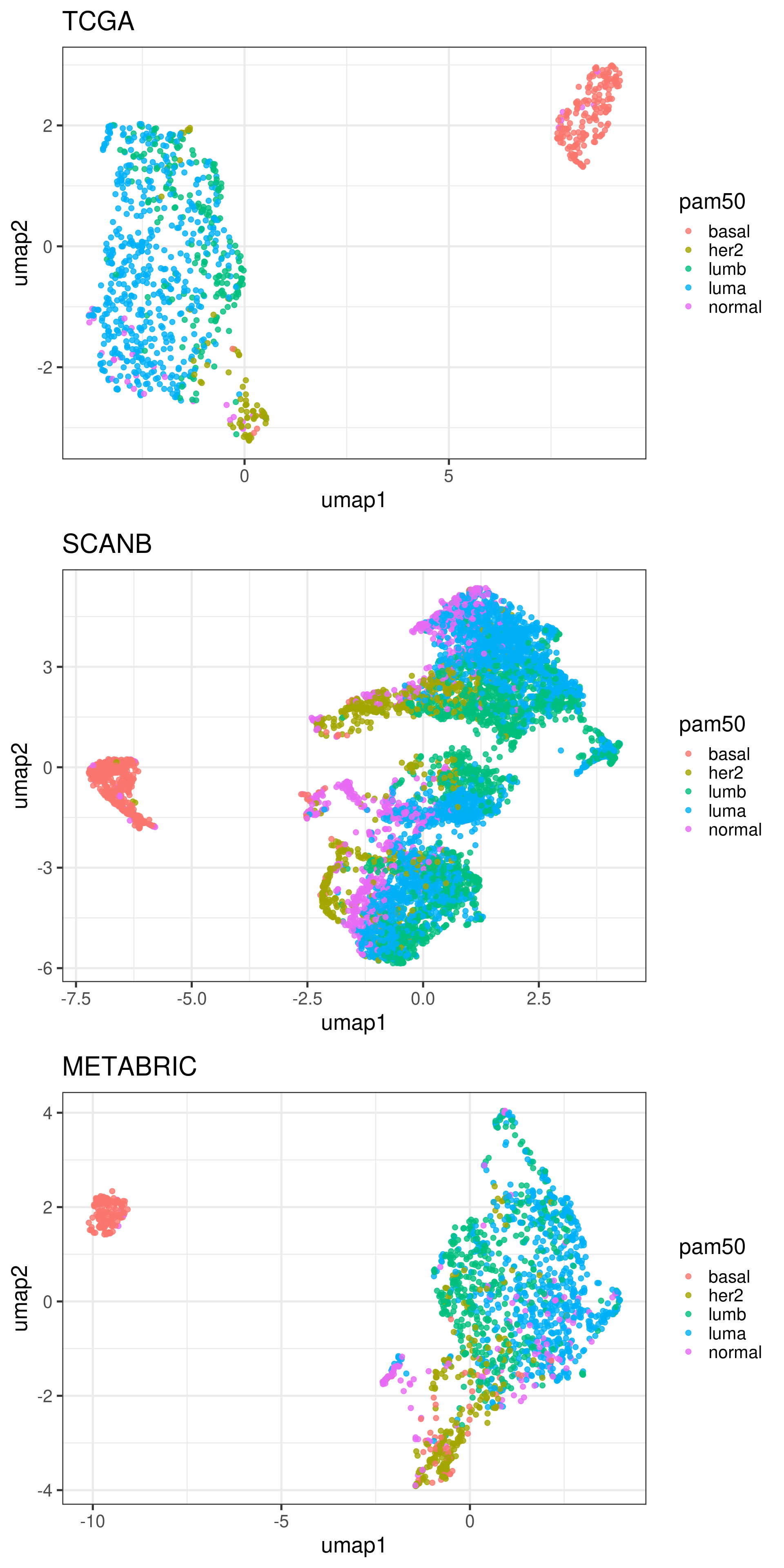
The plots below show how each patient is different in a molecular sense, and even inside each molecular subtype there are some differences. We only do the umap of samples that have a molecular subtype assigned.

Figure 1.1: UMAP projections of all three cohorts in the following order”:” TCGA, SCANB and METABRIC. They are colored by the PAM50 molecular subtype.

From the plots above we see a distinction of the different molecular subtypes.

1.3 Calculating scores

In order to calculate the scores, the package msigdb is used to load the hallmark data into R. The \(SET_{ER/PR}\) is made of the following genes:

Affy	ID	is_target
202089_s_at	SLC39A6	yes
203438_at	STC2	yes
204508_s_at	CA12	yes
205225_at	ESR1	yes
205380_at	PDZK1	yes
205440_s_at	NPY1R	yes
205831_at	CD2	yes
206401_s_at	MAPT	yes
209123_at	QDPR	yes
209309_at	AZGP1	yes
209459_s_at	ABAT	yes
213245_at	ADCY1	yes
213539_at	CD3D	yes
214440_at	NAT1	yes
218398_at	MRPS30	yes
218976_at	DNAJC12	yes
219197_s_at	SCUBE2	yes
222379_at	KCNE4	yes
200650_s_at	LDHA	no
202961_s_at	ATP5J2	no
211662_s_at	VDAC2	no
201623_s_at	DARS	no
205480_s_at	UGP2	no
217750_s_at	UBE2Z	no
212175_s_at	AK2	no
212050_at	WIPF2	no
202631_s_at	APPBP2	no
202342_s_at	TRIM2	no

The first 18 genes are considered to be the target genes, the last 10 genes are the genes used for reference. According to their paper, the score is calculated in the following way:

\[ SET_{ER/PR} = \sum_{i = 1}^{18} \frac{T_i}{18} - \sum_{j=1}^{10}\frac{R_j}{10} + 2 \]

Where \(T_i\) are the expression levels of target genes and \(R_j\) are the expression levels of the reference genes. Here we use GSVA to calculate the scores, even when using their genes.

Before we calculate any score, let us check the number of genes available for each pathway in each dataset. This is important, in other to have robust scores, most of the genes should be available in the datasets. We also add signatures of 18 and 200 random genes for control.

pathway	tcga	scanb	metabric	n	average_percentage
HALLMARK_ADIPOGENESIS	188	187	164	210	0.86
HALLMARK_ALLOGRAFT_REJECTION	141	134	139	335	0.41
HALLMARK_ANDROGEN_RESPONSE	93	92	83	102	0.88
HALLMARK_ANGIOGENESIS	30	29	28	36	0.81
HALLMARK_APICAL_JUNCTION	155	148	151	231	0.66
HALLMARK_APICAL_SURFACE	31	30	31	46	0.67
HALLMARK_APOPTOSIS	141	141	130	183	0.75
HALLMARK_BILE_ACID_METABOLISM	75	71	77	114	0.65
HALLMARK_CHOLESTEROL_HOMEOSTASIS	67	67	60	77	0.84
HALLMARK_COAGULATION	92	90	88	162	0.56
HALLMARK_COMPLEMENT	152	149	144	237	0.63
HALLMARK_DNA_REPAIR	145	144	127	170	0.82
HALLMARK_E2F_TARGETS	196	179	174	218	0.84
HALLMARK_EPITHELIAL_MESENCHYMAL_TRANSITION	179	172	172	204	0.85
HALLMARK_ESTROGEN_RESPONSE_EARLY	189	176	162	216	0.81
HALLMARK_ESTROGEN_RESPONSE_LATE	176	162	162	218	0.76
HALLMARK_FATTY_ACID_METABOLISM	128	124	127	165	0.77
HALLMARK_G2M_CHECKPOINT	187	172	173	204	0.87
HALLMARK_GLYCOLYSIS	173	167	167	215	0.79
HALLMARK_HEDGEHOG_SIGNALING	24	21	25	36	0.65
HALLMARK_HEME_METABOLISM	152	150	138	214	0.69
HALLMARK_HYPOXIA	168	163	163	215	0.77
HALLMARK_IL2_STAT5_SIGNALING	163	156	163	216	0.74
HALLMARK_IL6_JAK_STAT3_SIGNALING	65	62	63	103	0.61
HALLMARK_INFLAMMATORY_RESPONSE	142	131	144	222	0.63
HALLMARK_INTERFERON_ALPHA_RESPONSE	92	90	81	140	0.63
HALLMARK_INTERFERON_GAMMA_RESPONSE	178	176	164	286	0.6
HALLMARK_KRAS_SIGNALING_DN	71	54	82	220	0.31
HALLMARK_KRAS_SIGNALING_UP	156	147	146	220	0.68
HALLMARK_MITOTIC_SPINDLE	194	189	168	215	0.85
HALLMARK_MTORC1_SIGNALING	190	189	176	211	0.88
HALLMARK_MYC_TARGETS_V1	194	194	185	236	0.81
HALLMARK_MYC_TARGETS_V2	58	57	52	60	0.93
HALLMARK_MYOGENESIS	126	131	139	212	0.62
HALLMARK_NOTCH_SIGNALING	29	28	29	34	0.84
HALLMARK_OXIDATIVE_PHOSPHORYLATION	199	185	169	220	0.84
HALLMARK_P53_PATHWAY	177	172	160	215	0.79
HALLMARK_PANCREAS_BETA_CELLS	14	13	17	44	0.33
HALLMARK_PEROXISOME	85	84	87	110	0.78
HALLMARK_PI3K_AKT_MTOR_SIGNALING	91	91	84	118	0.75
HALLMARK_PROTEIN_SECRETION	94	92	90	98	0.94
HALLMARK_REACTIVE_OXYGEN_SPECIES_PATHWAY	46	47	43	58	0.78
HALLMARK_SPERMATOGENESIS	62	59	71	144	0.44
HALLMARK_TGF_BETA_SIGNALING	49	50	45	59	0.81
HALLMARK_TNFA_SIGNALING_VIA_NFKB	175	173	166	228	0.75
HALLMARK_UNFOLDED_PROTEIN_RESPONSE	106	106	98	115	0.9
HALLMARK_UV_RESPONSE_DN	129	131	121	152	0.84
HALLMARK_UV_RESPONSE_UP	129	126	127	191	0.67
HALLMARK_WNT_BETA_CATENIN_SIGNALING	36	33	36	50	0.7
HALLMARK_XENOBIOTIC_METABOLISM	142	135	141	224	0.62
SET_ERPR	18	16	16	18	0.93
random_200	156	131	148	200	0.72
random_18	14	12	14	18	0.74

Most of the genes are available in all datasets. When calculating scores it is always good to check the availability of the genes. Otherwise this can make the score unstable, since too many of the genes are missing. For example, HALLMARK_PANCREAS_BETA_CELLS might have an unstable score, due to a lot of genes missing.

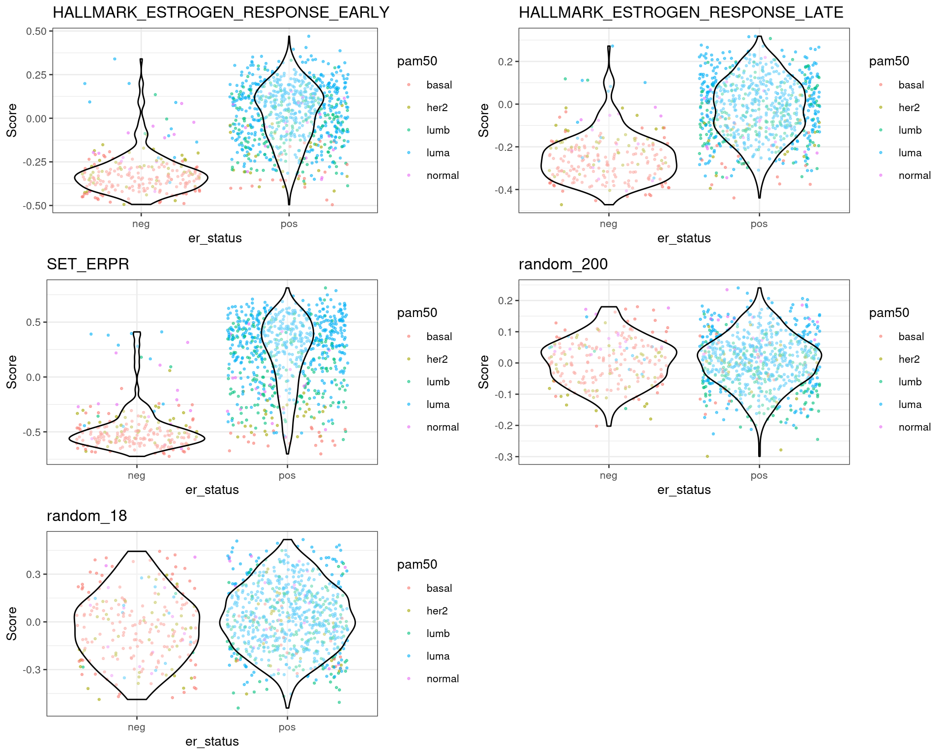
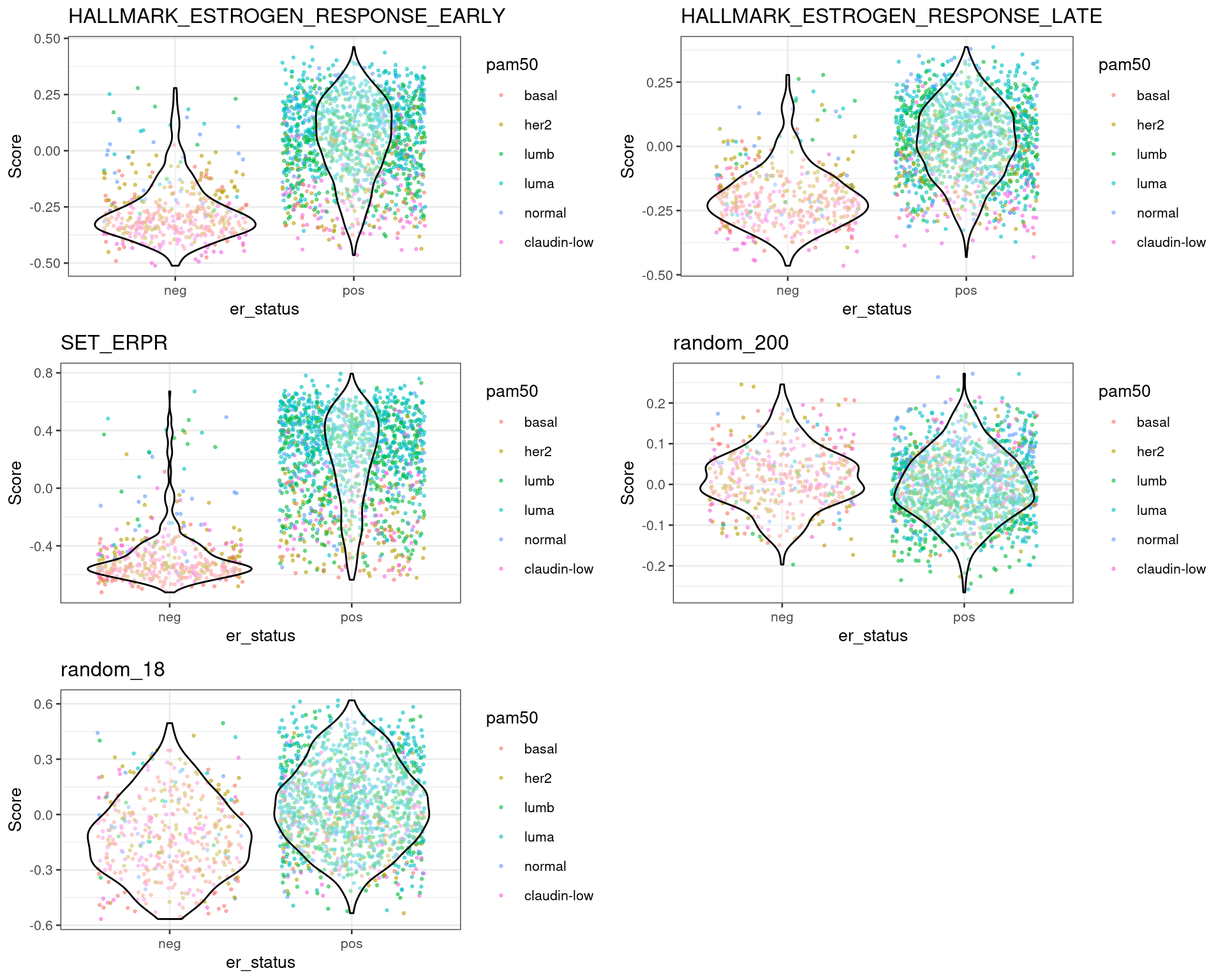
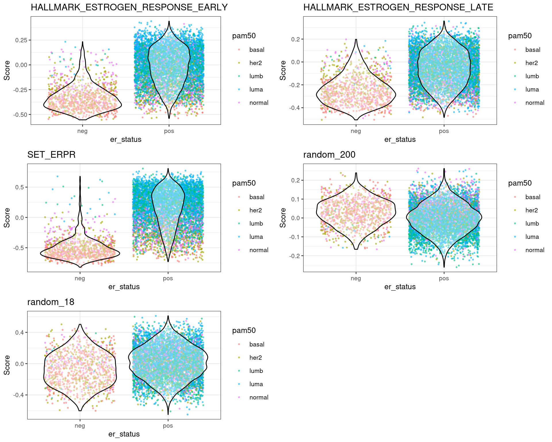
For each dataset one can plot the differences in scores for ER+ and ER- BC patients. This should be already an indication that the scores are meaningful. The next sections shows the results for each dataset individually.

TCGA

Figure 1.2: Scores for TCGA patients

METABRIC

Figure 1.3: Scores for METABRIC patients

SCANB

Figure 1.4: Scores for SCANB patients

From the plots above one can conclude that three different estrogen pathways capture the differences between ER status and also molecular subtypes. There are two plots with random genes for control and we can see that there is no difference between the ER status when using those gene sets.

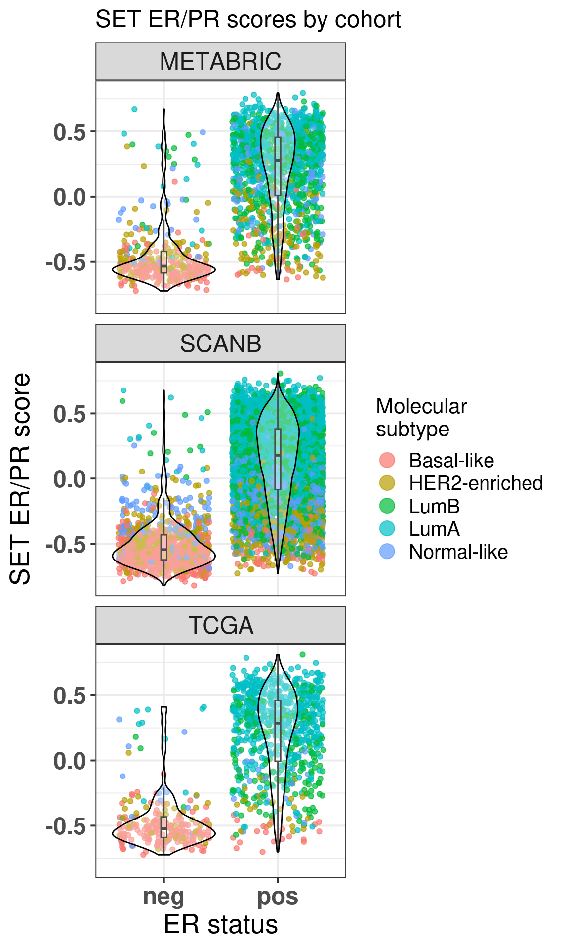
Below is a combined image for TCGA, SCANB and METABRIC using the \(SET_{ER/PR}\) signature.

Figure 1.5: SET ER/PR scores for all three cohorts.

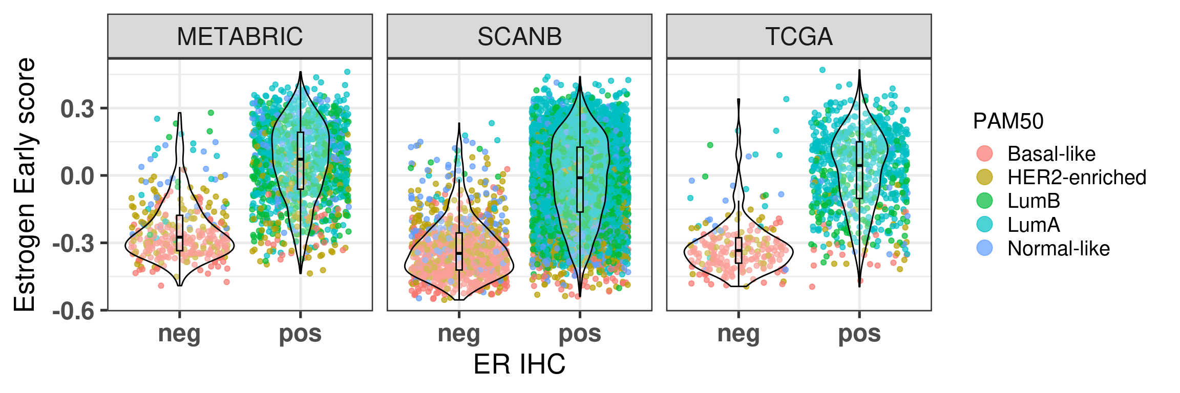
And now using the hallmark estrogen response early.

Figure 1.6: Estrogen early scores for all three cohorts.

We see that there is a considerable overlap between the ER+ and ER- BC samples. For each cohort the numbers of ER+ BC samples that have scores below 0 is shown below:

$metabric
                er_status                
 is_below_0           neg             pos
         no   6.04%  (20)  64.80%   (869)
        yes  93.96% (311)  35.20%   (472)
      Total 100.00% (331) 100.00% (1,341)

$scanb
                  er_status                
 is_below_0             neg             pos
         no   3.40%    (36)  48.27% (2,972)
        yes  96.60% (1,023)  51.73% (3,185)
      Total 100.00% (1,059) 100.00% (6,157)

$tcga
                er_status              
 is_below_0           neg           pos
         no   3.03%   (7)  57.49% (445)
        yes  96.97% (224)  42.51% (329)
      Total 100.00% (231) 100.00% (774)

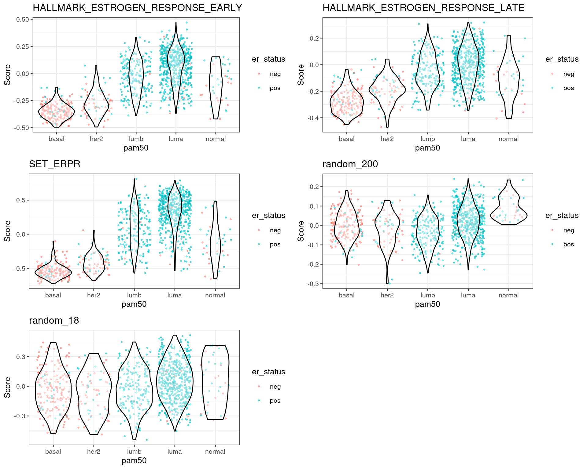
Another way to look at the data is to plot by molecular subtype instead of ER status.

TCGA

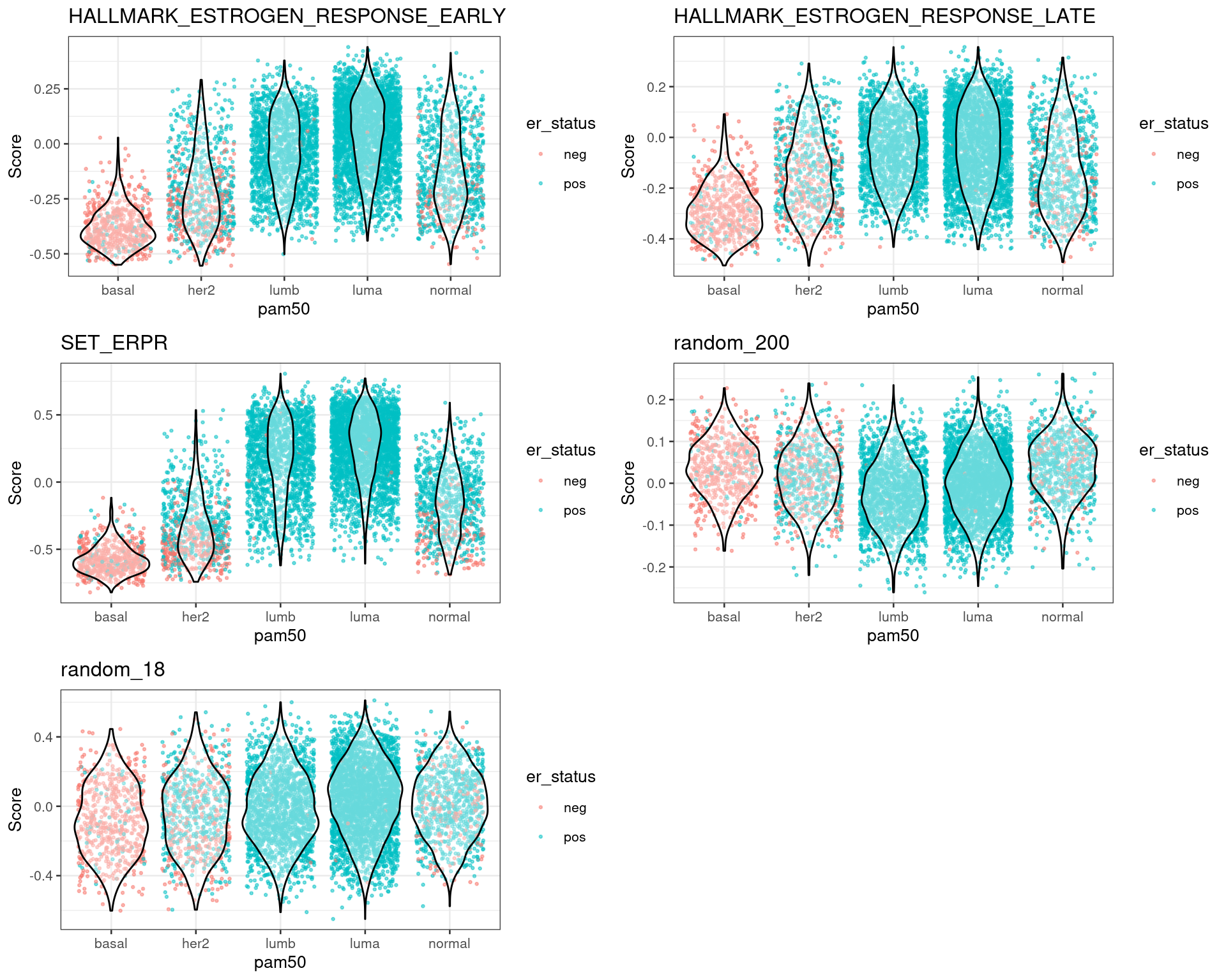
Figure 1.7: Scores for TCGA patients stratified by PAM50 molecular subtype

METABRIC

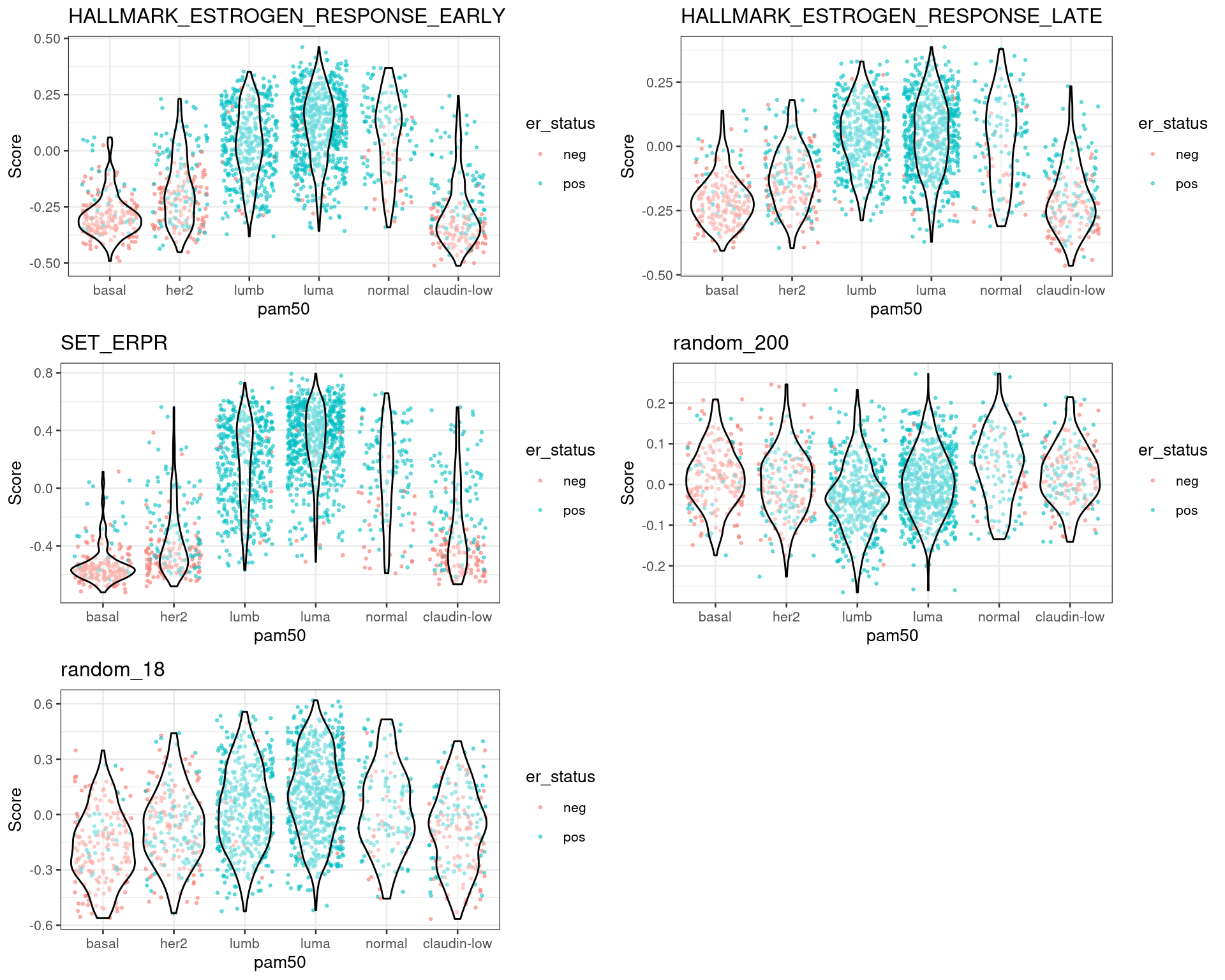
Figure 1.8: Scores for METABRIC patients stratified by PAM50 molecular subtype

SCANB

Figure 1.9: Scores for SCANB patients stratified by PAM50 molecular subtype

In all cohorts the luminal A and B patients have a similar score. Also the distinction is very clear between the basal and HER2-like patients versus luminal A and B.

One question that usually arises when calculating scores from gene sets is if proliferation associated genes (PAG) are driving the distinctions. These signatures are highly curated and they have close or no PAGs. Therefore, the scores are not affected by PAGs and they really reflect the biology.

Lastly we show in Figure 1.10 the correlation of the estrogen signaling scores with the signatures.

Figure 1.10: Scores for SCANB patients stratified by PAM50 molecular subtype

We see that there is a positive correlation between signatures and scores, the problem though is the high variability in the scores in this case.

In the next section we will show how these scores are also prognostic for ER+ BC patients.

1.4 Survival analysis

Since the scores are continuous variables and they are already scaled due to the output of GSVA, cox regression (Cox 1972) can be used. The advantages of using cox regression is that one can control for other variables. You might ask, why should one control for clinical variables? One of the reasons is because the data being dealt here is observational data. There are several confounders, for example, a score might be up because patients with a higher tumor grade have higher expression of some genes. Thus the score is confounded by the tumor grade and the interpretation changes.

There are limitations still when dealing with observational data. A strong hypothesis for performing survival analysis with observational data is that we have measured all the confounder variables. This is pretty strong and in practice we never know if a confounder is missing or not. For a more thorough overview of the causal framework for observational data, check the books (Gelman, Hill, and Vehtari 2020; McElreath 2020).

All the cohorts have a different set of clinical variables available. Therefore, the regression will be done by adjusting a different set of variables. Below is the description of the variables used for each cohort.¹

¹ This webpage explains with more details the different tumor stages and how BC are classified.

• Age: age is one of the most important factors to adjust, specially in breast cancer. This covariate is used for all cohorts.
• NPI: the Nottingham prognostic index scores each tumor based on tumor grade, tumor size and number of lymph nodes. Only METABRIC has this information.
• Tumor Size: as name describes. Only SCANB has this information.
• Tumor Stage: tumors are usually described in terms of stage, it reflects the tumor size and location. SCANB and TCGA have this information.
• Node Stage: similar to tumor stage, but encodes the number of lymph nodes where breast cancer cells can be found. SCANB and TCGA have this information.

Thus the models we are going to use for the survival analysis of each dataset is shown below.

• TCGA: ~ score + age + node_stage + tumor_stage,
• SCANB: ~ score + age + node_stage + tumor_stage,
• METABRIC: ~ score + age + NPI,

where score is one of the scores calculated earlier with GSVA. Note here that since each node stage and tumor stage have sub classifications they will be grouped together, otherwise there will be too many variables with few points. We will also subselect specific tumor stages for TCGA and SCANB, since there are very few patients with tumor stage 4.

To be very specific in the survival analysis, only endocrine treated patients should be used in the analysis, as that is what are interested in. METABRIC and SCANB has this kind of annotation, but TCGA not. So the survival analysis on SCANB and METABRIC will be performed on endocrine only treated, ER+ BC patients. On TCGA, to mitigate this effect, we subselect only luminal A and B patients, and we keep in mind that they might have been treated with chemotherapy as well. Moreover, in Sweden the guidelines for BC treatment is to use 10% as the threshold for ER status. Therefore, ER+ BC patients used on SCANB are those that are above the 10% threshold.

The table below shows the number of patients for each cohort.

cohort	number_patients	nb_events
TCGA	684	73
TCGA High ER	216	7
SCANB	3169	544
METABRIC	934	573
SCANB High ER	2542	399
SCANB Low ER	203	38
SCANB High ESR1	425	95
METABRIC High ESR1	254	175

The total number of HER2+ samples in the lists is:

cohort	number_patients	her2_positive
SCANB	3169	83
METABRIC	934	169

1.4.1 Results

The table below shows the results for each analysis performed for a specific term. In order to understand the table the user can filter based on the term, cohort and type of analysis. Since METABRIC has recurrence free survival (RFS) and overall survival (OS), the results for both analysis are presented here.

The table above shows that \(SET_{ER/PR}\) had a small hazard ratio (< 1) in all 4 analysis performed. Moreover, for all cases where a measure of estrogen signaling was used, the hazard ratio was below 1, indicating that the higher the score, the less likely the patient is to suffer the event in a specific timepoint. This indicates that ER signaling is actually something continuous and not dichotomous.

Not only that but we also performed Accelerated Failure Time (AFT) survival analysis with a log-normal distribution as our parametric distribution to model time. The results are shown in the table below.

And when using AFT analysis we see similar results. The estimates are on their scale (\(beta\)), meaning that values higher than 0 correspond to a slow down in the time to event. In this case here, if the estimate is higher than 0, then the time to death or time to recurrence is prolonged. In other words, estrogen signaling is associated with good outcome as well.

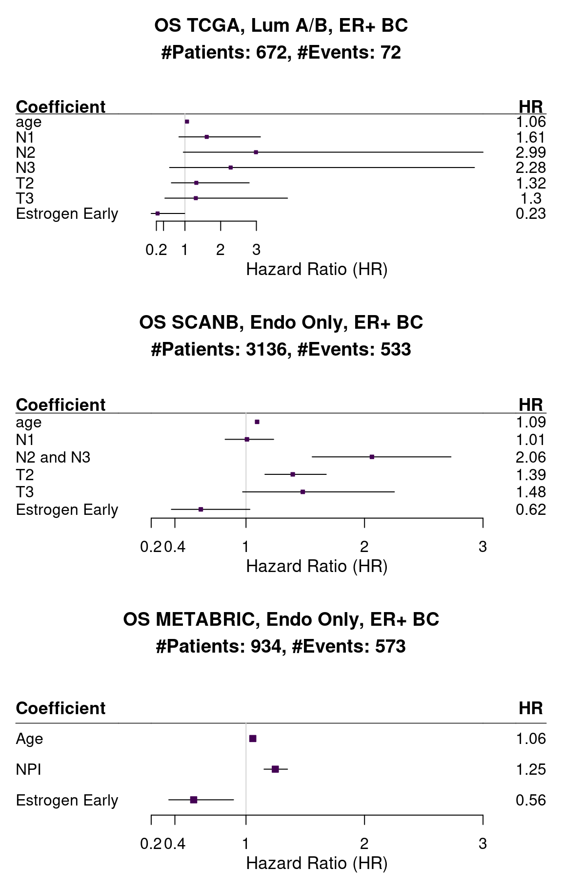
Figure 1.11 shows the forest plot of HALLMARK_ESTROGEN_RESPONSE_EARLY for all three cohorts.

Figure 1.11: Forest plots of the different cohorts and their hazard ratios. The bars correspond to 95% confidence interval.

The hazard ratios are all below 1 and small for HALLMARK_ESTROGEN_RESPONSE_EARLY. The variability changes depending on the cohort, specially because they have different follow-up times, SCANB being the shortest. TCGA has very few number of events and we could not select based on the treatment, the results for TCGA are less reliable.

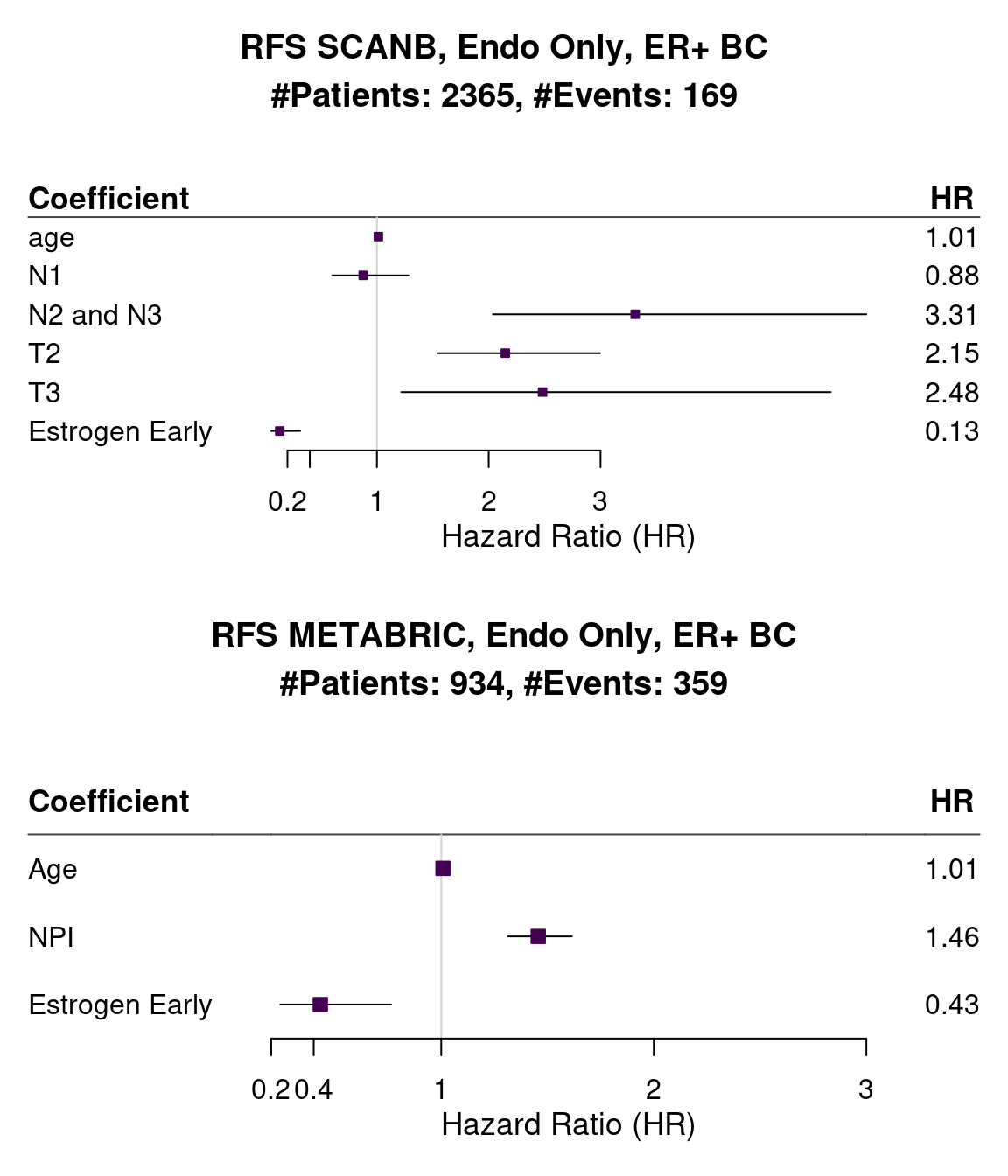
Below we show the results for recurrence free survival.

Figure 1.12: Forest plots of the different cohorts and their hazard ratios. The bars correspond to 95% confidence interval.

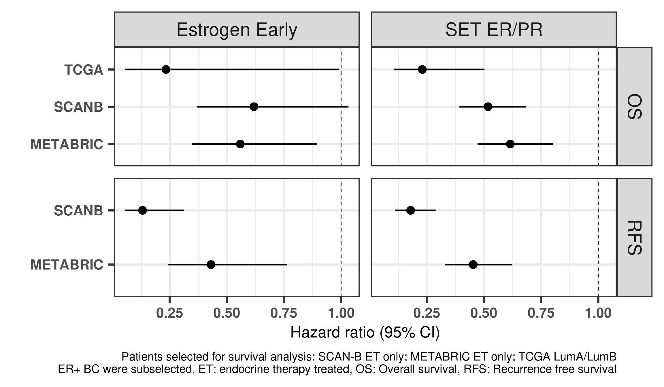
And Figure 1.13 is a different way of display the same results but only including the hazard ratios of the variables of interest.

Figure 1.13: Hazard ratios for estrogen early and SET ER/PR for all the three cohorts of only endocrine treated patients with ER+ BC.

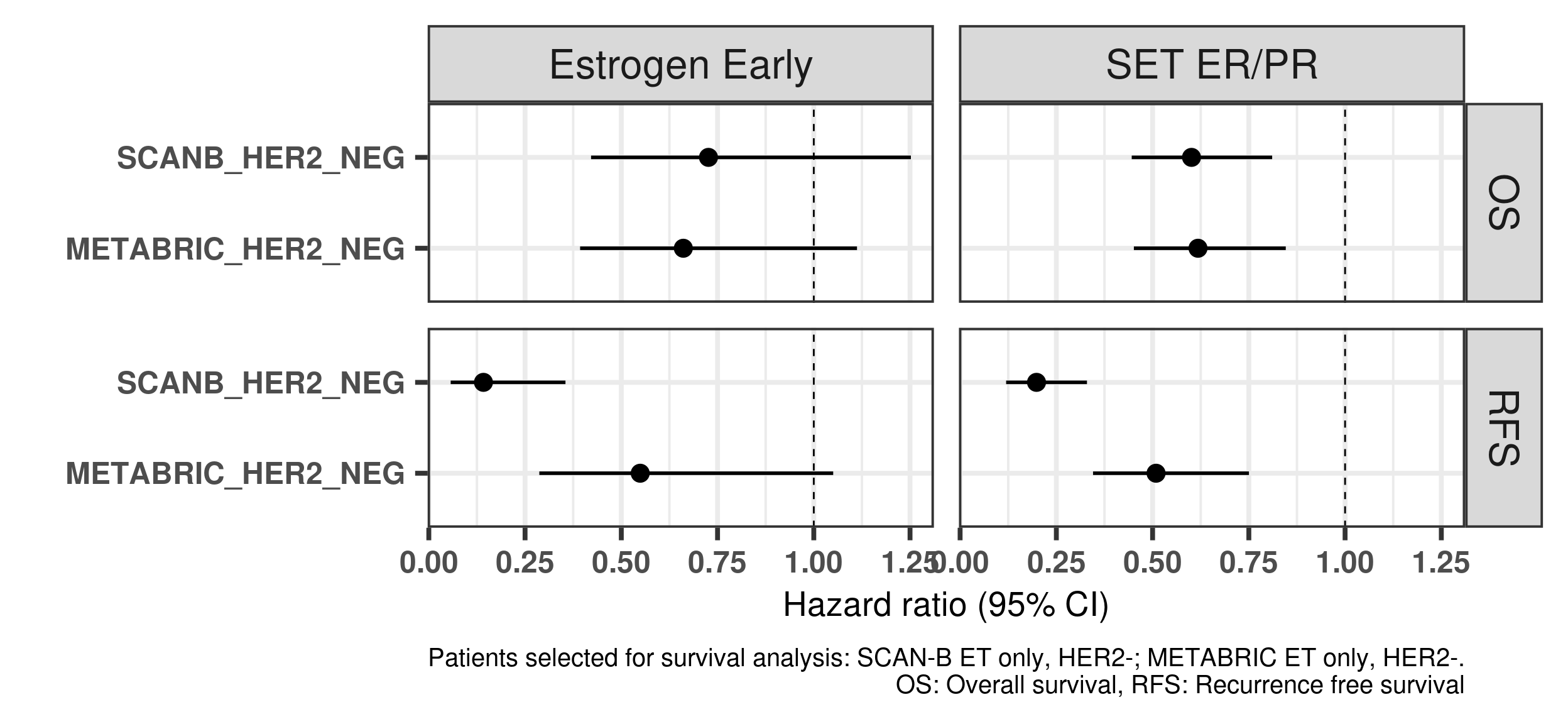
And now including only SCANB and METABRIC using the HER2- samples only.

Figure 1.14: Hazard ratios for estrogen early and SET ER/PR for all the three cohorts of only endocrine treated patients with ER+ HER2- BC.

Below we show the correlation between estrogen response early and SET ER/PR using the ER+ HER2- BC samples.

    Pearson's product-moment correlation

data:  colData(datasets$scanb)[scanb_samples_her2_neg, "HALLMARK_ESTROGEN_RESPONSE_EARLY"] and colData(datasets$scanb)[scanb_samples_her2_neg, "SET_ERPR"]
t = 30.347, df = 3034, p-value < 2.2e-16
alternative hypothesis: true correlation is not equal to 0
95 percent confidence interval:
 0.4547881 0.5093842
sample estimates:
      cor 
0.4825548 

    Pearson's product-moment correlation

data:  colData(datasets$metabric)[metabric_samples_her2_neg, "HALLMARK_ESTROGEN_RESPONSE_EARLY"] and colData(datasets$metabric)[metabric_samples_her2_neg, "SET_ERPR"]
t = 22.125, df = 763, p-value < 2.2e-16
alternative hypothesis: true correlation is not equal to 0
95 percent confidence interval:
 0.5799848 0.6665138
sample estimates:
      cor 
0.6251665 

In general they are positively correlated but not to the extreme.

1.5 Comparison of ER IHC and molecular ER signaling

The new released dataset from the SCANB consortium contains the ER percentage based on the IHC stainings. This is great, because we can now compare the molecular ER signaling score to what is seen in the clinics.

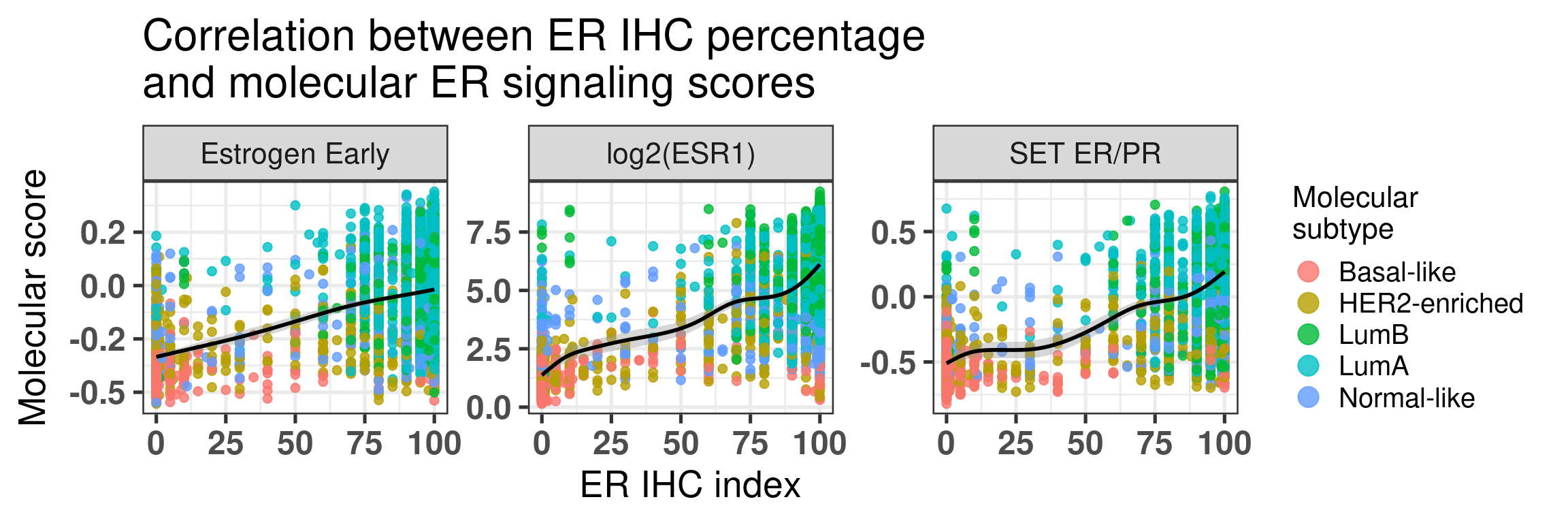
First we start by comparing the molecular score with the percentages (Figure 1.15).

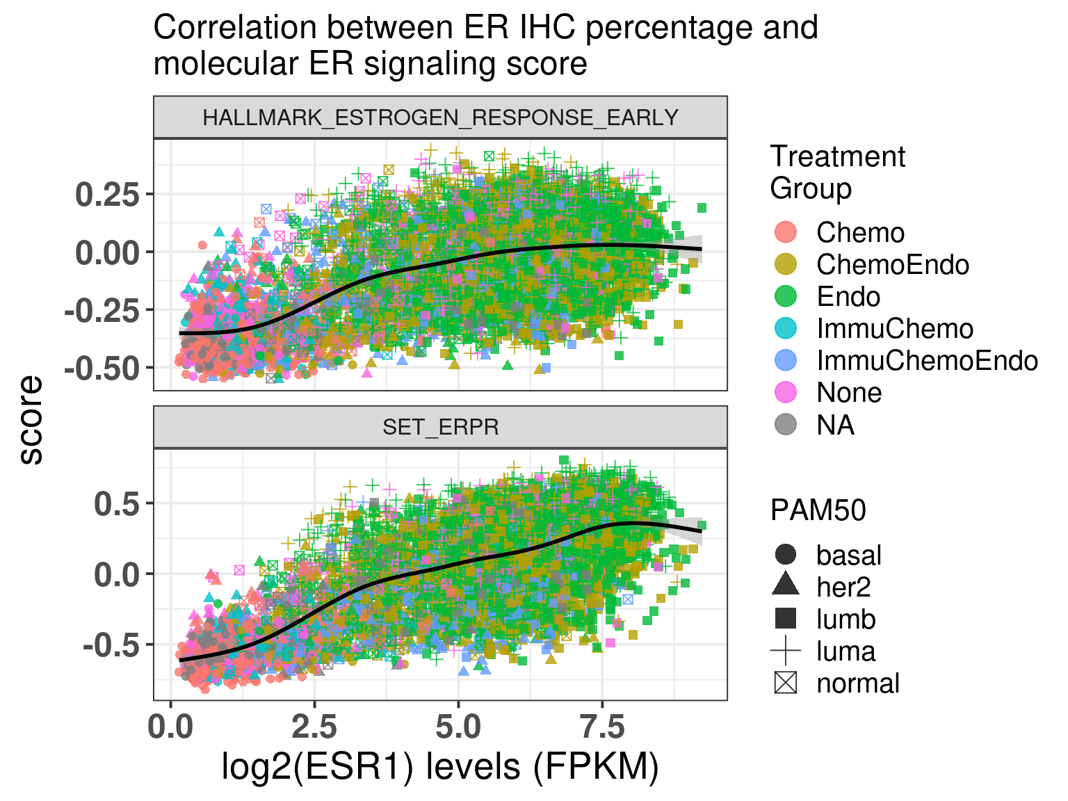
Figure 1.15: Correlation between ER IHC percentage and molecular ER signaling by using the signature HALLMARK_ESTROGEN_RESPONSE_EARLY and SET ER/PR.

The first thing that one can notice is that ER percentage is very discrete, pathologists probably don’t assign non rounded percentage values, which makes sense. Another thing to notice is that for high ER percentage patients you have a whole spectrum of molecular ER signaling score.

The spearman correlation for Estrogen early and ER IHC is:

    Spearman's rank correlation rho

data:  df_wide$ER.pct and df_wide$HALLMARK_ESTROGEN_RESPONSE_EARLY
S = 2.4797e+10, p-value < 2.2e-16
alternative hypothesis: true rho is not equal to 0
sample estimates:
     rho 
0.389119 

For SET ER/PR is:

    Spearman's rank correlation rho

data:  df_wide$ER.pct and df_wide$SET_ERPR
S = 1.9706e+10, p-value < 2.2e-16
alternative hypothesis: true rho is not equal to 0
sample estimates:
      rho 
0.5145412 

And finally for log(ESR1) is:

    Spearman's rank correlation rho

data:  df_wide$ER.pct and df_wide$`log2(ESR1)`
S = 1.7107e+10, p-value < 2.2e-16
alternative hypothesis: true rho is not equal to 0
sample estimates:
      rho 
0.5785603 

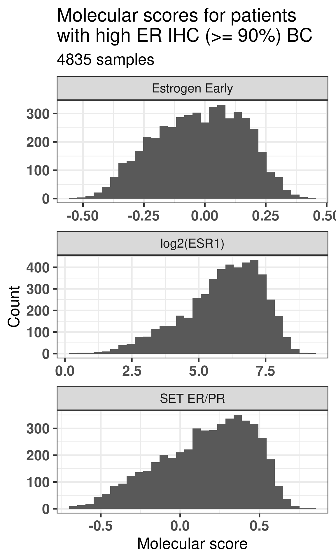
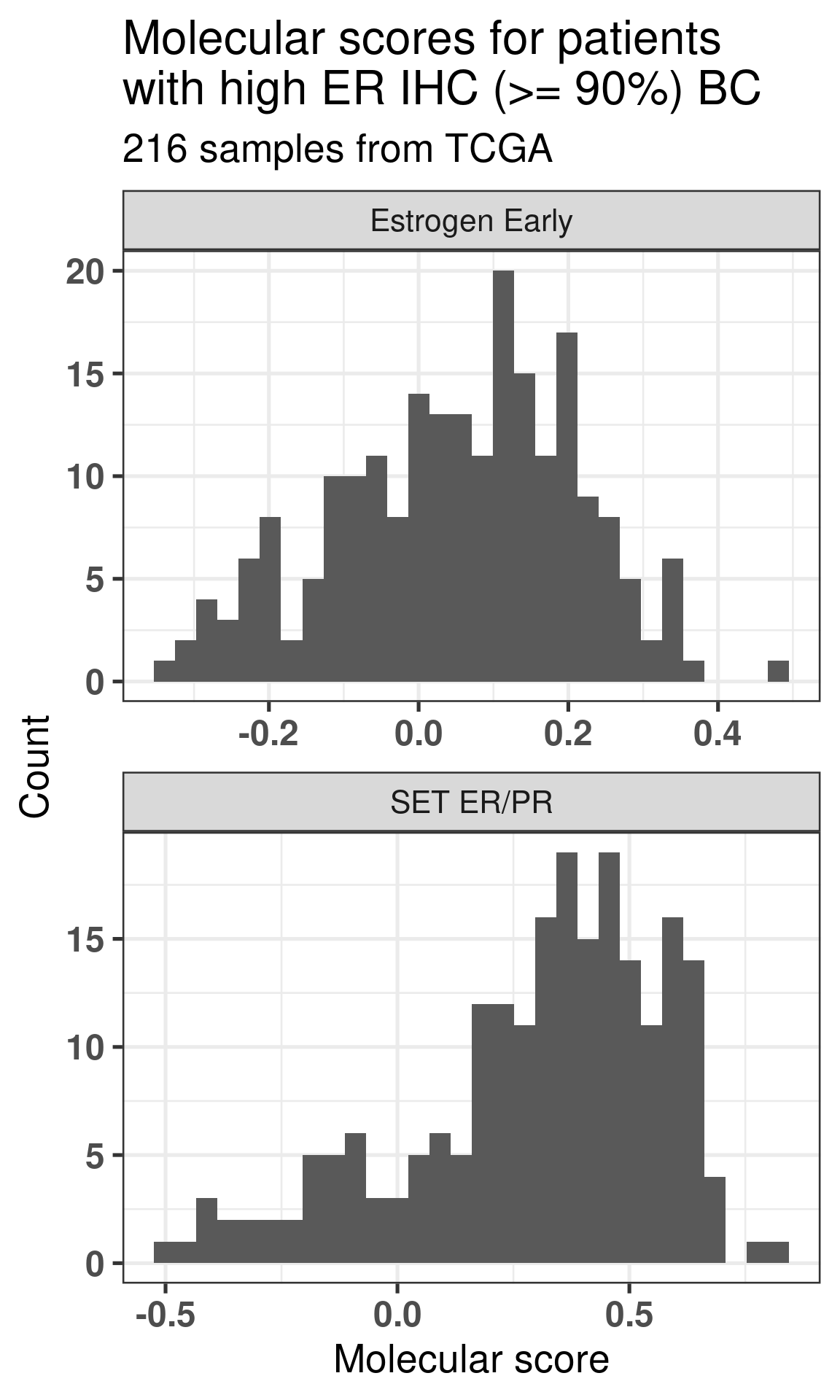
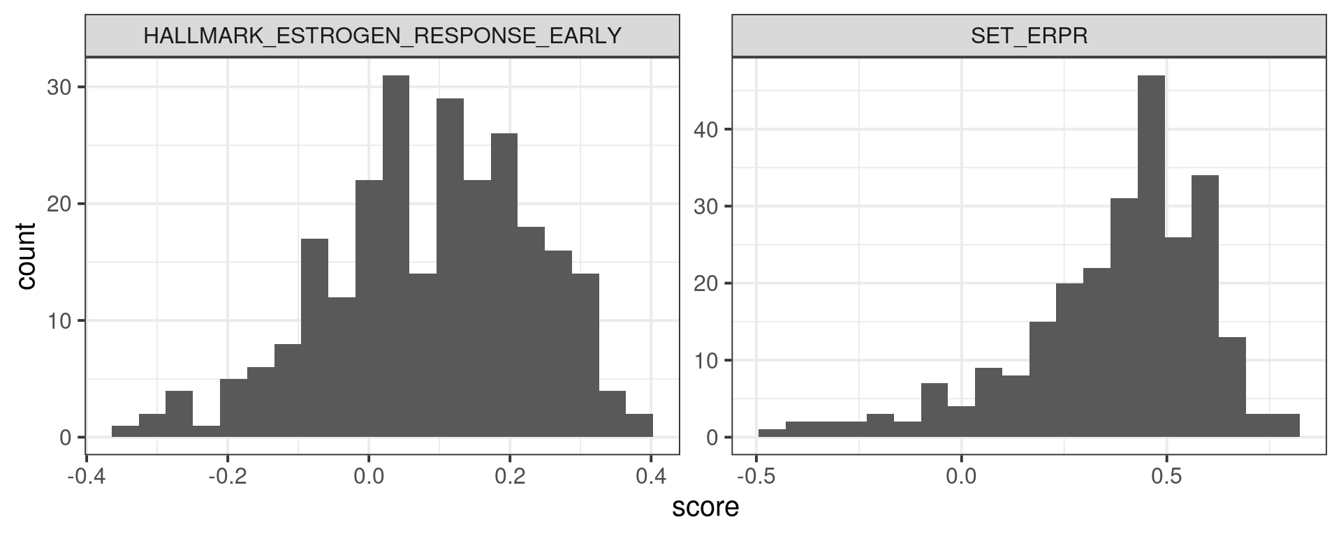
Now we look speficially at the high ER percentage patients and compare their ER signaling scores. We previously saw that the distribution of these scores seems to be wide.

Figure 1.16: Scores for high ER percentage breast cancer patients.

Figure 1.16 shows how the distributions are not skewed towards high values only. It looks like there is a step in the SET ER/PR signature, we now compare with the ESR1 values and hallmark estrogen response early.

Figure 1.17: Scores for high ER percentage breast cancer patients.

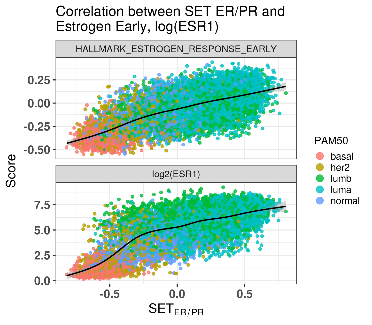
Figure 1.18: Correlation between SET ER/PR and other scores.

There is a highly positive correlation. Also interesting to see that ESR1 levels are not necessarily highly correlated with high SET ER/PR scores. Remember that for ESR1 the scale is logarithmic, so even if the slope is smaller than in the hallmark estrogen response early, it might mean a higher correlation even.

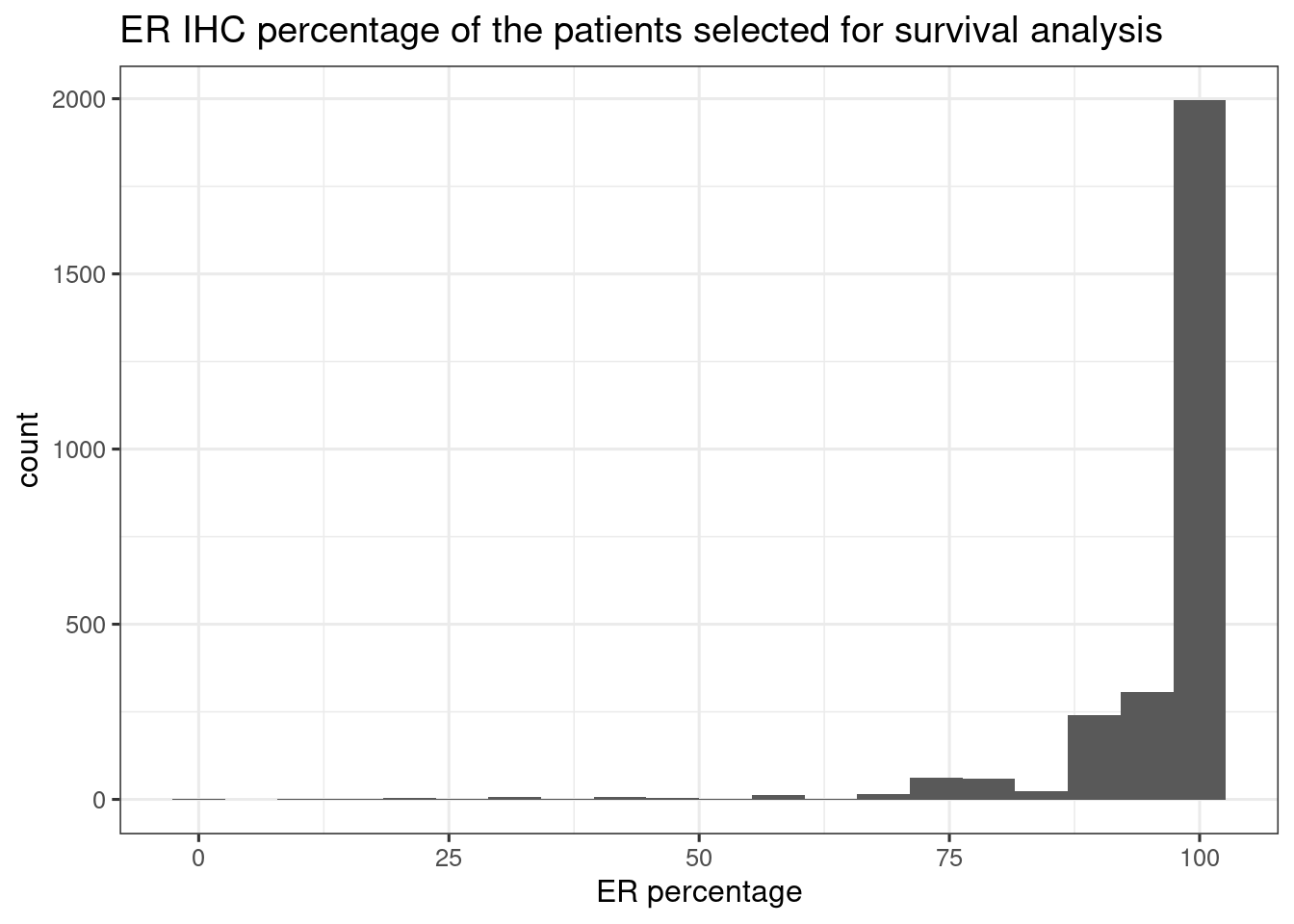
Figure 1.19 shows the distribution of the ER IHC percentage for the patients used in the previous survival analysis for SCANB.

Figure 1.19: Histogram of ER IHC percentage of the SCANB samples used for survival analysis

We see that the majority of the patients actually have already pretty high percentage. It could be that the results of the overall survival analysis are actually driven by the the low ER percentage patients, so we performed the survival analysis only on patients with ER percentage equal or higher than 90%. The table below shows the total number of patients for each analysis.

cohort	number_patients	nb_events
TCGA	684	73
TCGA High ER	216	7
SCANB	3169	544
METABRIC	934	573
SCANB High ER	2542	399
SCANB Low ER	203	38
SCANB High ESR1	425	95
METABRIC High ESR1	254	175

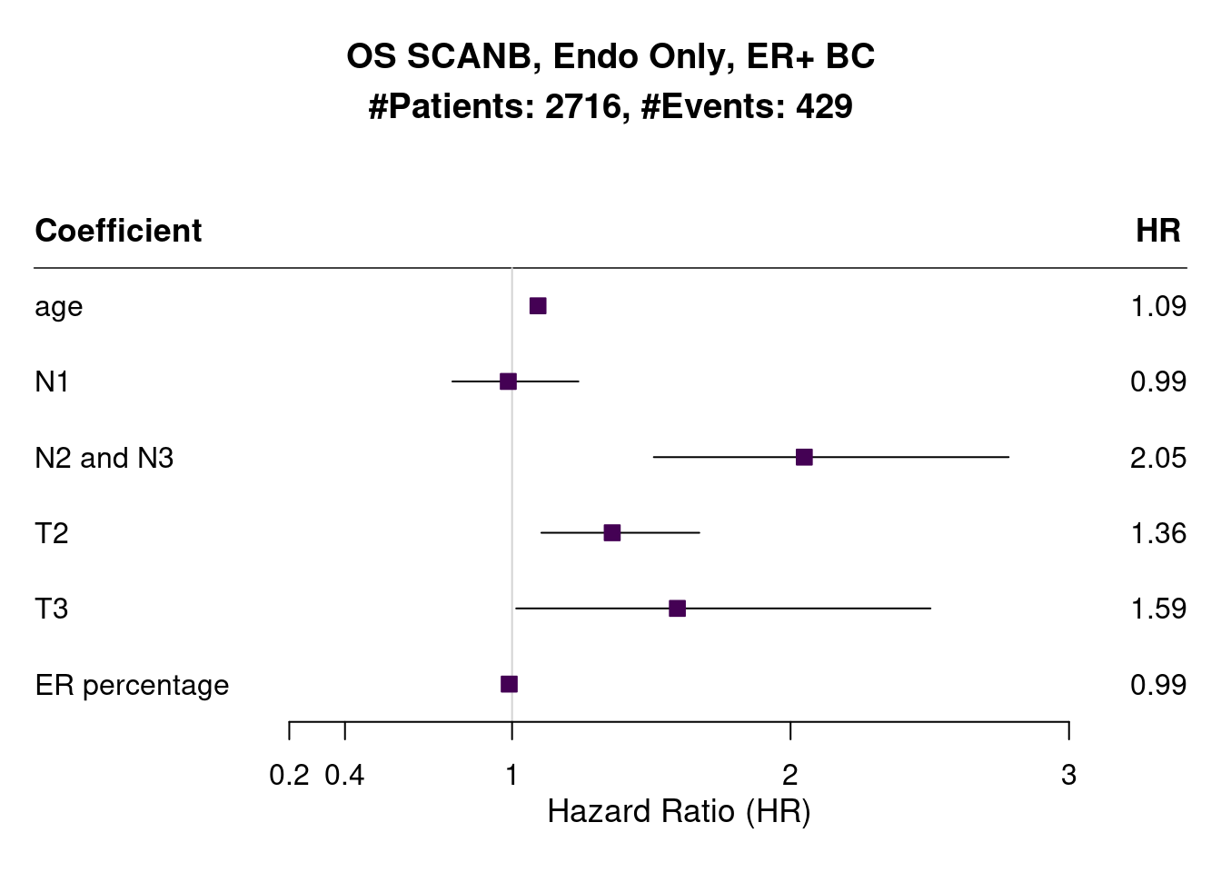
There was a decrease of around 200 patients with 80 events less, so indeed a lot of those patients with lower ER percentage had died. Figure 1.20 shows the results of the survival analysis when considering the ER IHC percentage as a continuous score on SCANB.

Figure 1.20: Survival analysis using ER IHC percentage as the score instead of the common molecular ER signaling scores

We a very tight confidence interval in this case with a HR very close to 1, meaning that for every 1% increase there is a 2% decrease in your risk of dying. The table with the values is shown below.

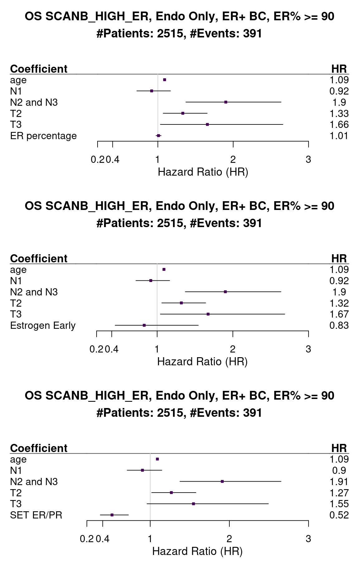
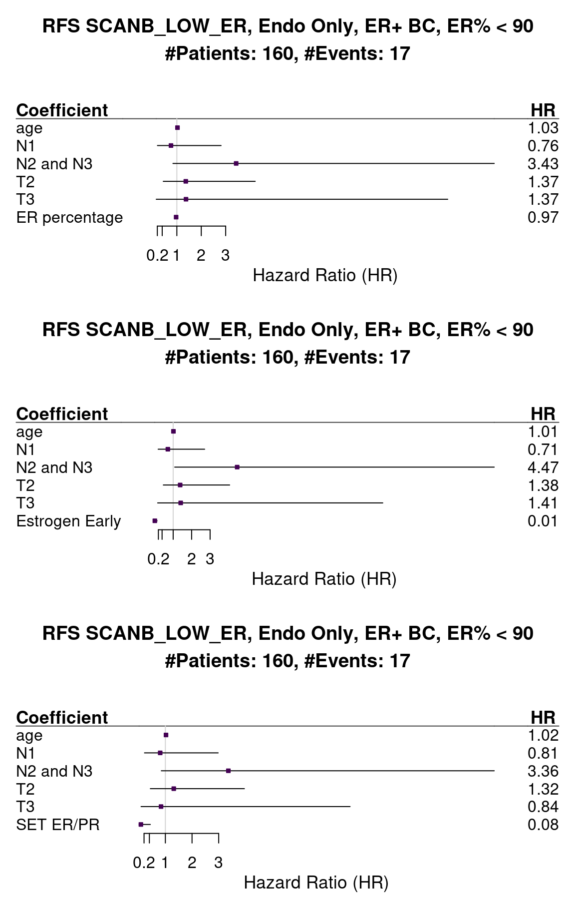
Next we selected only patients that had 90% or more ER IHC percentage to perform the survival analysis. Figure 1.21 shows the results for both the analysis done on ER IHC percentage,
HALLMARK_ESTROGEN_RESPONSE_EARLY and SET_ERPR.

Figure 1.21: Survival analysis using ER IHC percentage, HALLMARK_ESTROGEN_RESPONSE_EARLY and SET_ERPR as the scores. Only patients with 90% or more in the ER IHC were selected.

When performing the survival analysis among the high ER percentage, there is no evidence to differentiate between 90 to 100%, but by using the molecular scores that fact is still true, showing that perhaps the molecular score could be more sensitive for these patients.

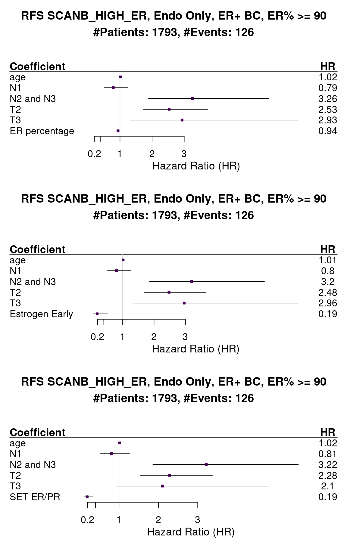
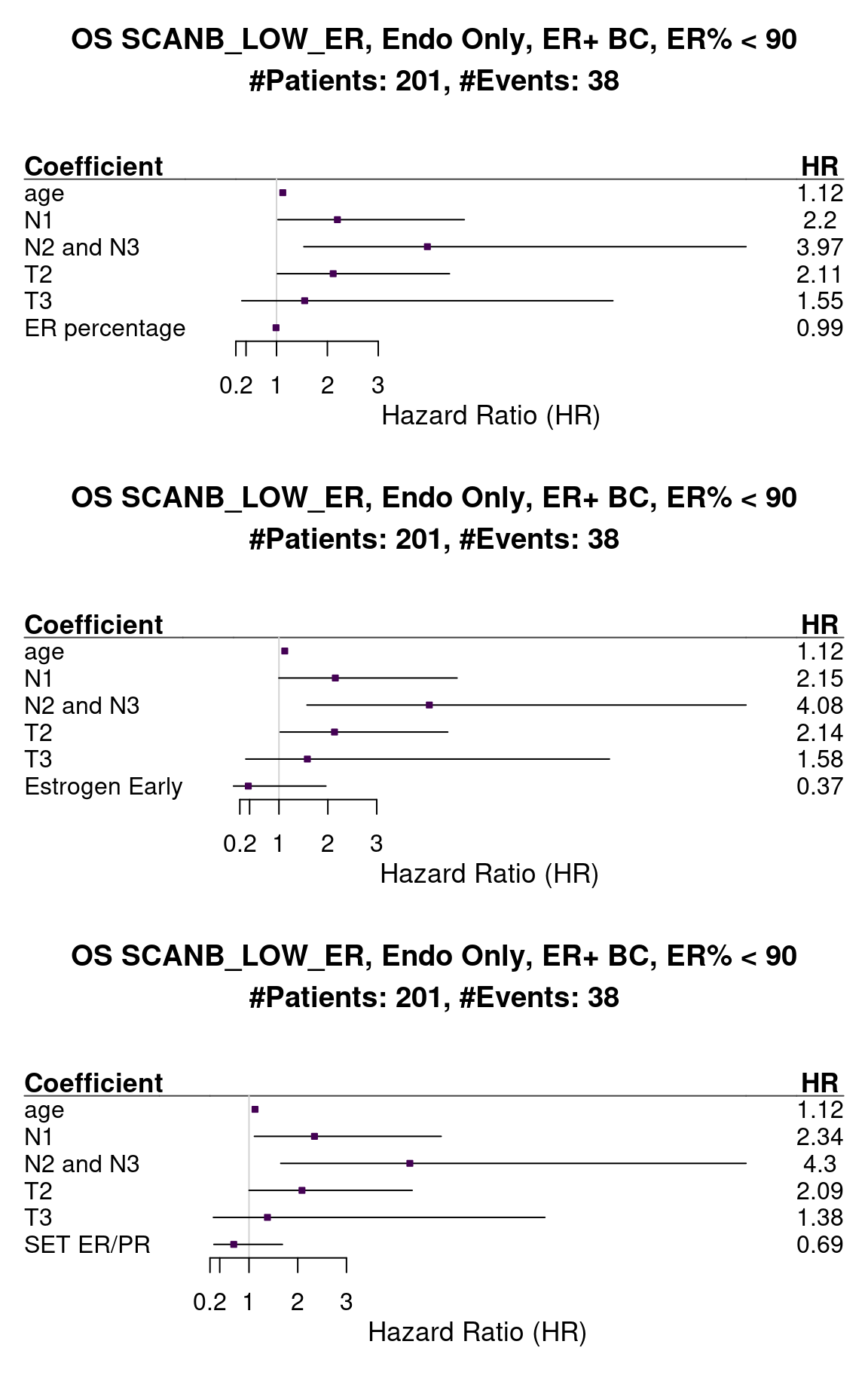
We can also analyse the recurrence free survival for this cohort (Figure 1.22).

Figure 1.22: Survival analysis using ER IHC percentage, HALLMARK_ESTROGEN_RESPONSE_EARLY and SET_ERPR as the scores. Only patients with 90% or more in the ER IHC were selected.

The problem now is that the number of events is much smaller, so the confidence intervals for the estimates will be bigger. We see that for both signatures the HR is way below 1, meaning that the higher the score the better it is for the patient. Also the hazard ratio decreased in this case.

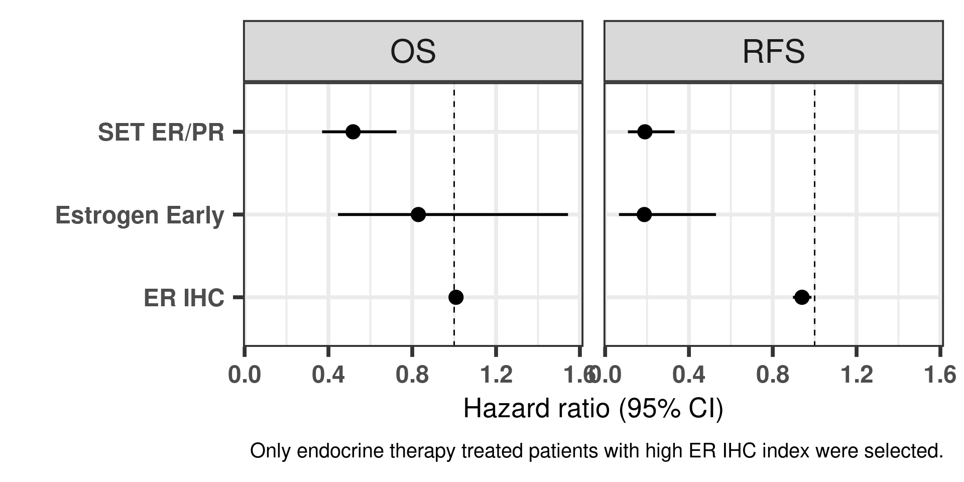
Another way of visualizing as previously is shown below (Figure 1.23).

Figure 1.23: Hazard ratios for estrogen early and SET ER/PR for all the three cohorts of only endocrine treated patients with ER+ BC.

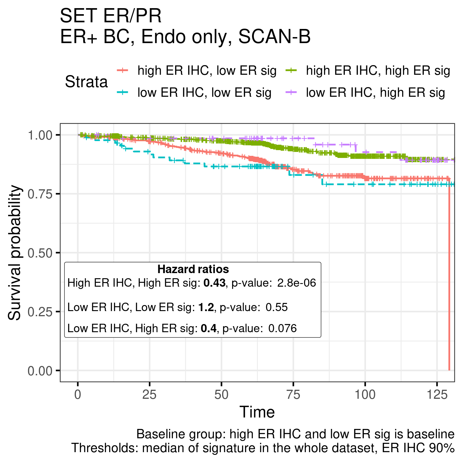
To further validate the ER signaling we partitionate the score in 4 different categories, low, intermediate, high, ultra high and perform the OS and RFS analysis.

For SET ER/PR the results are:

Call:
survival::coxph(formula = Surv(rfs_months, rfs_status) ~ sig_dich + 
    age + node_stage + tumor_stage, data = df)

                                 coef exp(coef)  se(coef)      z        p
sig_dichhighERIHC_highERsig -0.843412  0.430240  0.179931 -4.687 2.77e-06
sig_dichlowERIHC_lowERsig    0.184400  1.202496  0.309776  0.595   0.5517
sig_dichlowERIHC_highERsig  -0.920174  0.398450  0.518530 -1.775   0.0760
age                          0.019260  1.019447  0.008289  2.324   0.0201
node_stageN1                -0.236426  0.789444  0.215939 -1.095   0.2736
node_stageN2and3             1.140900  3.129585  0.255540  4.465 8.02e-06
tumor_stageT2                0.835757  2.306559  0.185411  4.508 6.56e-06
tumor_stageT3                0.787449  2.197782  0.386906  2.035   0.0418

Likelihood ratio test=106.7  on 8 df, p=< 2.2e-16
n= 1953, number of events= 143 
   (1216 observations deleted due to missingness)

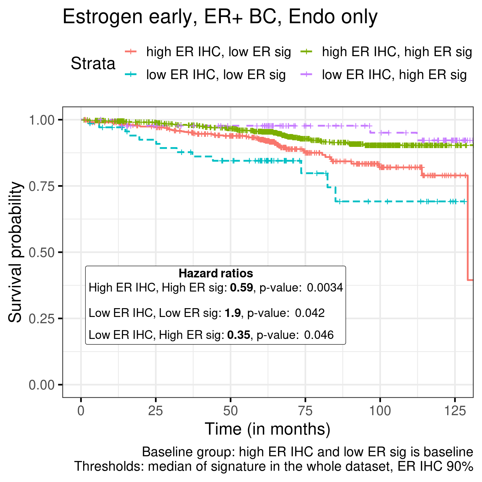
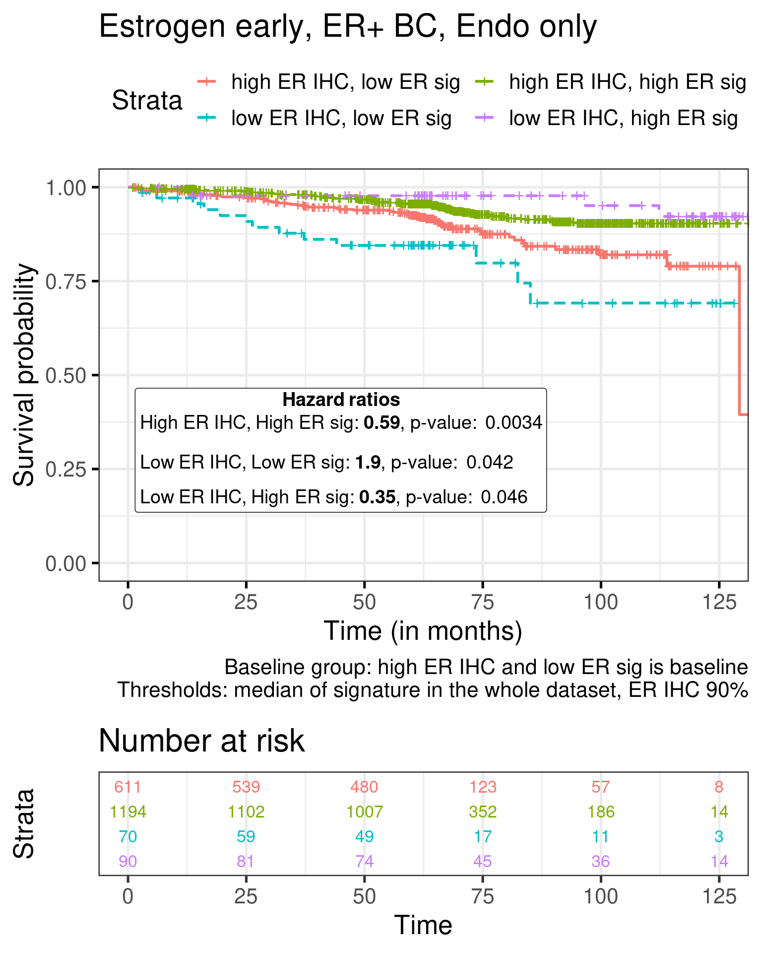
For Estrogen early the results are:

Call:
survival::coxph(formula = Surv(rfs_months, rfs_status) ~ sig_dich + 
    age + node_stage + tumor_stage, data = df)

                                 coef exp(coef)  se(coef)      z        p
sig_dichhighERIHC_highERsig -0.526967  0.590393  0.180072 -2.926  0.00343
sig_dichlowERIHC_lowERsig    0.630550  1.878643  0.310235  2.032  0.04210
sig_dichlowERIHC_highERsig  -1.057145  0.347446  0.530040 -1.994  0.04610
age                          0.017054  1.017200  0.008363  2.039  0.04144
node_stageN1                -0.208378  0.811900  0.216655 -0.962  0.33615
node_stageN2and3             1.215071  3.370533  0.258466  4.701 2.59e-06
tumor_stageT2                0.830548  2.294575  0.186152  4.462 8.13e-06
tumor_stageT3                0.910210  2.484843  0.382392  2.380  0.01730

Likelihood ratio test=99.35  on 8 df, p=< 2.2e-16
n= 1953, number of events= 143 
   (1216 observations deleted due to missingness)

High ER sig and high ER IHC have a better outcome than high ER IHC and low ER sig for both signatures.

The table below shows the number of RFS events for each subgroup in the SET ER/PR dichotomization procedure.

                         rfs_status                            
            sig_dich              1           2           Total
  highERIHC_lowERsig 88.04%   (508) 11.96% (69) 100.00%   (577)
 highERIHC_highERsig 95.11% (1,168)  4.89% (60) 100.00% (1,228)
   lowERIHC_lowERsig 85.39%    (76) 14.61% (13) 100.00%    (89)
  lowERIHC_highERsig 94.37%    (67)  5.63%  (4) 100.00%    (71)

Next we show the Kaplan Meier estimate curves for both signatures.

Figure 1.24: Kaplan-Meier estimate of the categorized SET ER/PR signature

Figure 1.25: Kaplan-Meier estimate of the categorized Estrogen early signature

And including the number of events.

In both cases there is a good distinction between low ER sig/High ER IHC and High ER sig/Low ER IHC. Interestingly, there the worst group is really the low ER sig/low ER IHC, as expected.

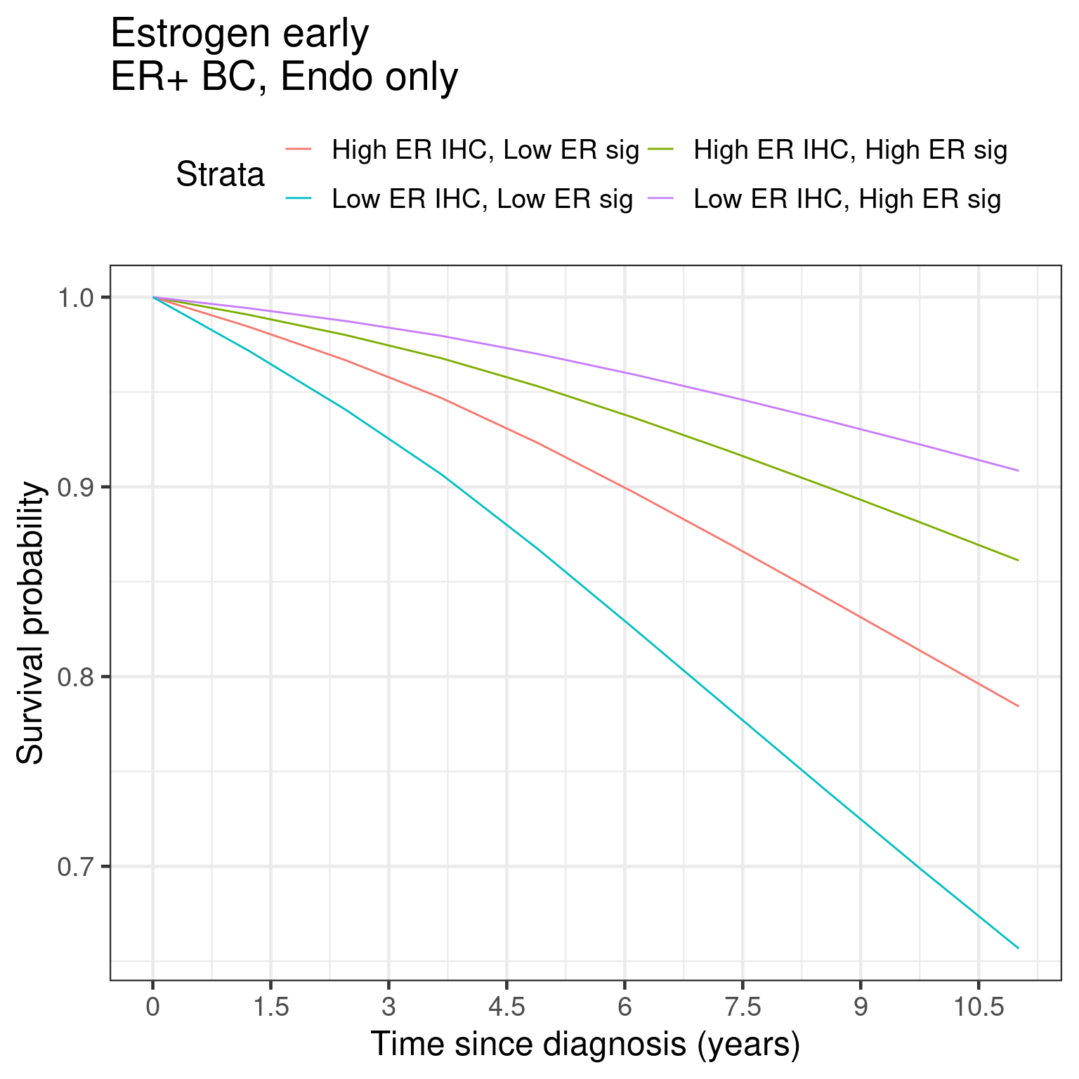
We can do a similar analysis now using the marginal survival curves from the package flexsurv along with the functions flexsurvspline and standsurv.

First we show the marginal RFS curves.

Figure 1.26

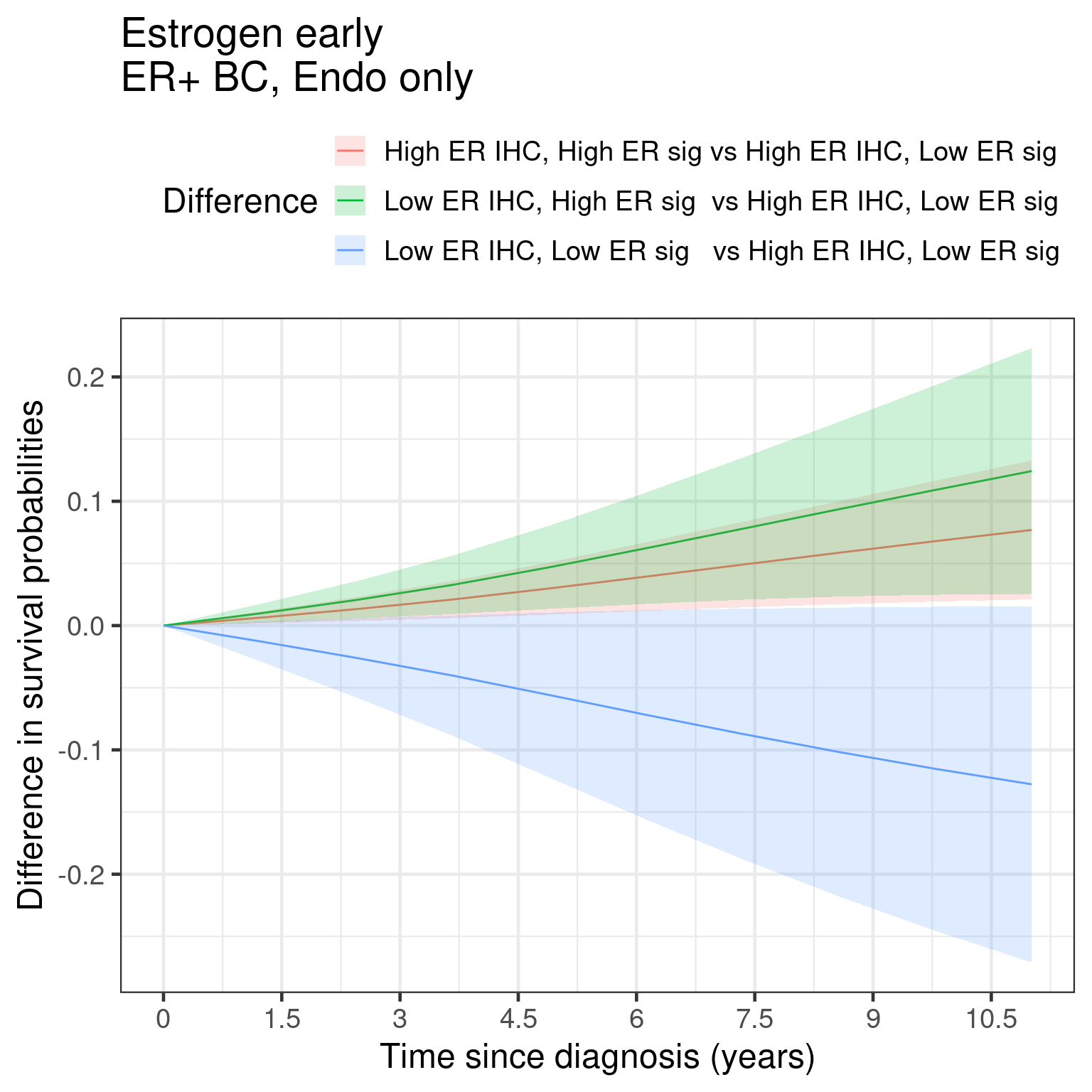
And now the marginal curves for the differences.

Figure 1.27

We see similar things to the KM as done before. But here now we are using the standardized survival curves.

We now evaluate the protective effect of the estrogen signaling signatures in the patients that have tumors with ER IHC lower than 90%.

Figure 1.28: Survival analysis using ER IHC percentage, HALLMARK_ESTROGEN_RESPONSE_EARLY and SET_ERPR as the scores. Only patients with less than 90% in the ER IHC were selected.

The number of patients now is very low, but the effect is still there. When we look at the survival. Below we show the results for the overall survival.

Figure 1.29: Survival analysis using ER IHC percentage, HALLMARK_ESTROGEN_RESPONSE_EARLY and SET_ERPR as the scores. Only patients with less than 90% in the ER IHC were selected.

The hazard ratio is still below 1 but the uncertainty is much higher, probably due to the number of patients and events.

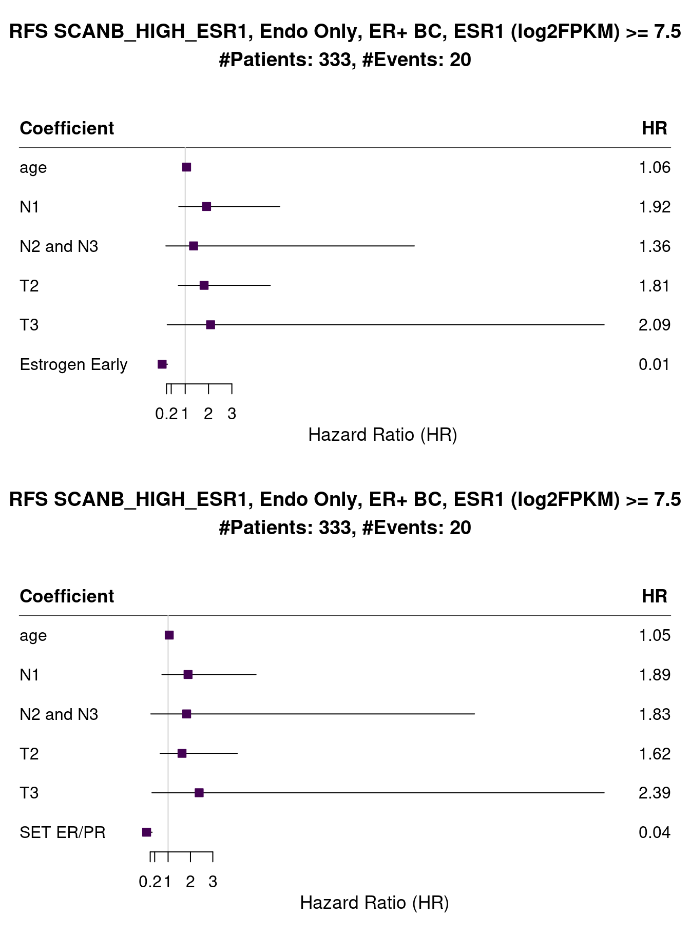
Another way of evaluating the effect of estrogen signaling and not only the presence of the estrogen receptor protein or the mRNA transcripts, is to check the patients whose tumor samples have high expression of ESR1. We can perform such analysis in both METABRIC and SCANB.

Figure 1.30: Survival analysis using ER IHC percentage, HALLMARK_ESTROGEN_RESPONSE_EARLY and SET_ERPR as the scores. Only patients with more than 7.5 units of ESR1 in the logFPKM scale were selected.

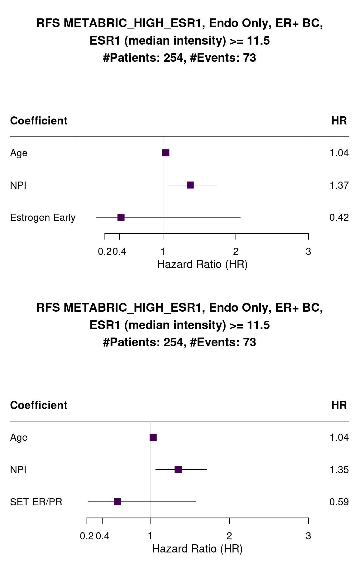
The number of events is very small but the HR is very small also and confidence interval is far away from 1. And now for METABRIC when we select all patients of 3rd quantile and above (median intensity higher than 11.5).

Figure 1.31: Survival analysis using HALLMARK_ESTROGEN_RESPONSE_EARLY and SET_ERPR as the scores. Only patients with more than 11 units of ESR1 in the log median intensity scale were selected.

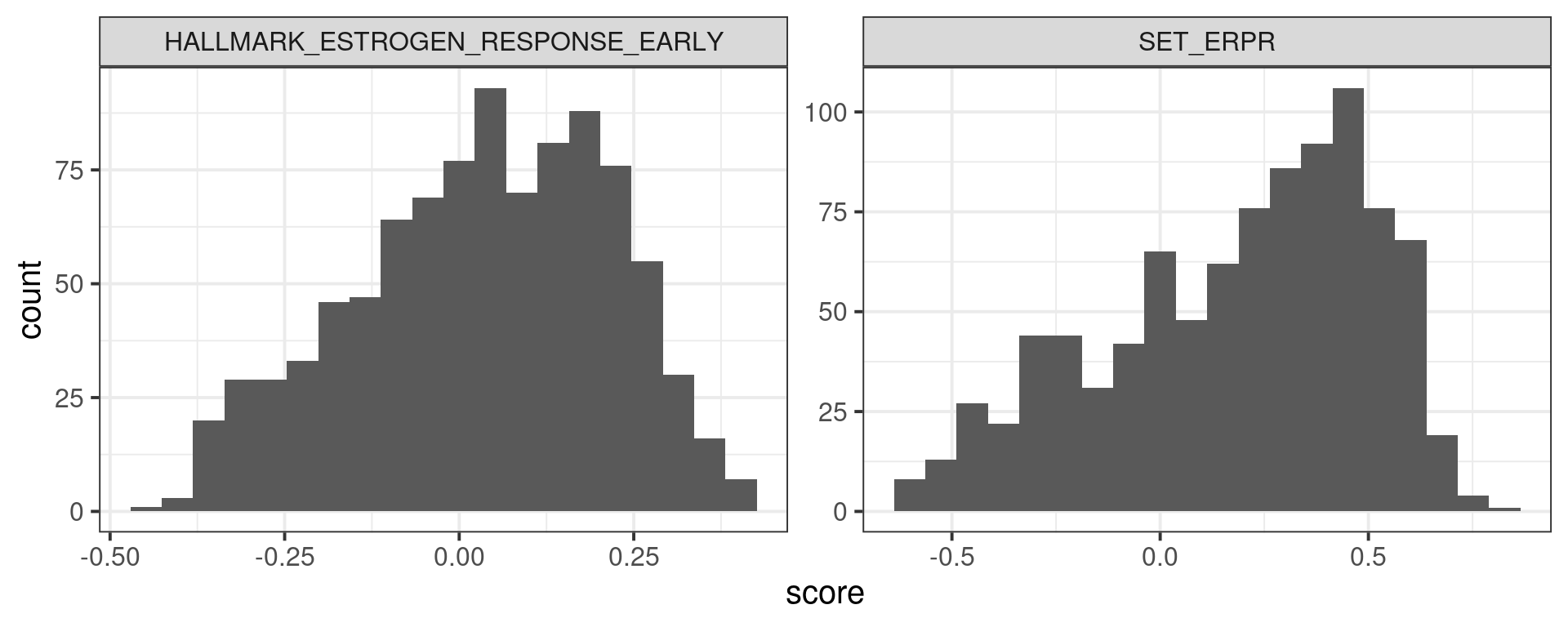
The variability is way higher but the hazard ratio is still below 1 as expected. In this case probably there are patients that have low score and don’t benefit as much from the treatment. Figure 1.32 shows the distribution of ER signaling scores for those patients. We notice that the average is very close to the peak of the distributions.

Figure 1.32

And below for all patients used for the full analysis on METABRIC.

Figure 1.33

1.6 Conclusion

In this chapter we’ve shown that ER+ BC patients are very distinct from each other, as it can be seen from the umap projections and the subtypes. These patients might respond differently for endocrine therapy as well, and this might depend on the ER signaling, how active it is. Therefore, when deciding a treatment, more care should be taken with ER+ BC patients and check their signaling scores somehow. The \(SET_{ER/PR}\) signature is a good signature showing very good hazard ratios across the different cohorts. This signature has also been validated on the clinics for use.

Knowing the ER signaling for a patient is very important when deciding treatment, but not enough. What could be other alternatives for patients that have low ER signaling and are still considered ER+? Should they use only endocrine therapy or supplement it with something else? In the next chapters we present a framework where we can take a look at a more personalised approach for treatments.

Cox, D. R. 1972. “Regression Models and Life-Tables.” Journal of the Royal Statistical Society: Series B (Methodological) 34 (2): 187–202. https://doi.org/10.1111/j.2517-6161.1972.tb00899.x.

Gelman, Andrew, Jennifer Hill, and Aki Vehtari. 2020. Regression and Other Stories. Analytical Methods for Social Research. Cambridge, England: Cambridge University Press.

Hänzelmann, Sonja, Robert Castelo, and Justin Guinney. 2013. “GSVA: Gene Set Variation Analysis for Microarray and RNA-Seq Data.” BMC Bioinformatics 14 (1). https://doi.org/10.1186/1471-2105-14-7.

McElreath, Richard. 2020. Statistical Rethinking. 2nd ed. Chapman & Hall/CRC Texts in Statistical Science. London, England: CRC Press.

Sinn, Bruno V., Chunxiao Fu, Rosanna Lau, Jennifer Litton, Tsung-Heng Tsai, Rashmi Murthy, Alda Tam, et al. 2019. “SETER/PR: A Robust 18-Gene Predictor for Sensitivity to Endocrine Therapy for Metastatic Breast Cancer.” Npj Breast Cancer 5 (1). https://doi.org/10.1038/s41523-019-0111-0.

Subramanian, Aravind, Pablo Tamayo, Vamsi K. Mootha, Sayan Mukherjee, Benjamin L. Ebert, Michael A. Gillette, Amanda Paulovich, et al. 2005. “Gene Set Enrichment Analysis: A Knowledge-Based Approach for Interpreting Genome-Wide Expression Profiles.” Proceedings of the National Academy of Sciences 102 (43): 15545–50. https://doi.org/10.1073/pnas.0506580102.